 Prateek Gupta
Pipeline Parallelism
Toy setting to understand Tensor Parallelism.
This is the third part of the Distributed Training for Dummies series.
The code for this series is available in the Distributed Training For Dummies GitHub repository. The design of much of the code is inspired by the picotron library. While the code itself contains detailed comments, here I will walk through key code blocks to provide a quick and basic understanding of how to implement some distributed training techniques. To start setting up the environment, you can visit the GitHub repository or follow the detailed walkthrough here.
Note: There are highly efficient libraries available, such as Megatron and DeepSpeed, which are specifically optimized for distributed training. I recommend using them whenever possible.
Reference section in the book: Explore HuggingFace’s Pipeline Parallelism section here.
Quick Primer on Pipeline Parallelism
Pipeline Parallelism (PP) involves splitting a large language model (LLM) into groups of layers, with each group assigned to a different GPU. As a result, the outputs of one group (both forward activations and backward gradients) must be sent to the next worker in the pipeline.
Idle Time: Pipeline Bubbles. A key challenge in PP is that a process cannot compute the backward pass until it receives gradients from subsequent layers. This dependency can cause GPUs to sit idle, waiting for data—this idle time is known as the pipeline bubble.
Microbatches to keep the pipeline busy. To reduce idle time, the input batch is split into microbatches—smaller sets of samples processed independently. By processing microbatches in a staggered fashion, each GPU can continue working while communicating (activations or gradients), thus improving hardware utilization.
Scheduling to minimize pipeline bubble. The way microbatches are scheduled across GPUs has a significant impact on efficiency. Various scheduling schemes have been developed to maximize hardware utilization and minimize pipeline bubbles. Some notable approaches include:
- Integer Linear Programming (ILP) Schedules:
The authors of Zero Bubble Pipeline Parallelismformulated the scheduling problem as an ILP, deriving optimal and hand-crafted variants like ZB-H1 and ZB-H2 (see Appendix G of the paper). - Hand-Crafted Schedules:
Other labs have proposed their own schedules, such as DualPipe in the Deepseek-v3 Report, driving the bubble to 0.
Communication in Pipeline Parallelism. Despite the complexity of scheduling, the communication pattern in PP is relatively simple:
- Each GPU only needs to communicate with its immediate neighbor, sending activations or gradients as needed.
- This is a point-to-point (p2p) communication pattern.
Pipeline Parallelism in code
I found the implementation of these schedules to be quite confusing at first. To better understand them, I attempted to implement some myself, drawing heavily from the picotron library. In this post, I’ll walk through the design of the 1F1B schedule, using AFAB as a warmup to introduce the basics of pipeline parallelism. You can find the code here. To make the simulation more realistic, I’ve also added pseudo computation times to mimic the actual training scenario where each layer may take a substantial amount of time.
PiplineParallel Module
We simulate a large model composed of multiple layers—specifically linear layers in this example. Each layer is assigned to a different process using the distribute_layers() function, which ensures that each process holds only the layers relevant to its stage in the pipeline.
-
Forward pass: Computing the forward pass is straightforward. The
input_tensor—a microbatch for the first group or the output from the previous group for the rest—is passed through the local layers, producing anoutput_tensor. This output is then sent to the next group. -
Backward pass: The backward pass requires special handling of the
input_tensor. For every group after the first, theinput_tensorconsists of intermediate activations received from the previous stage. However, these tensors are not considered leaves in PyTorch’s computational graph and, by default, do not retain gradients.To enable backpropagation through the pipeline, we must explicitly call
retain_grad()oninput_tensor. Otherwise, callingtorch.autograd.backward(output_tensor, grad_tensors=output_tensor_grad)will fail to propagate gradients backward through the pipeline. Once gradients w.r.t.
input_tensorare computed, they must be sent to the previous GPU to continue the backward pass.
class PipelineParallel(torch.nn.Module):
    def __init__(self, model, pp_rank, pp_world_size):
        super().__init__()
        layer_distribution = self.distribute_layers(model.n_layers, pp_rank, pp_world_size)
        self.linear_layers = torch.nn.ModuleDict({str(i): model.linear_layers[i] for i in layer_distribution})
        self.final_layer = model.final_layer if pp_rank == pp_world_size - 1 else torch.nn.Identity()

    def distribute_layers(self, num_layers, pp_rank, pp_world_size):
        # layers_per_rank = num_layers // pp_world_size # this is even distribution
        # when the layers can't be distributed evenly, we add 1 to each available rank (starting from the first one)
        layers_per_rank = [num_layers // pp_world_size + (1 if i < num_layers % pp_world_size else 0) for i in range(pp_world_size)]
        start_layer = sum(layers_per_rank[:pp_rank])
        return range(start_layer, start_layer + layers_per_rank[pp_rank])

    def forward(self, input):
        x = input
        for layer in self.linear_layers.values():
            x = layer(x)
        return self.final_layer(x)

    def backward(self, input_tensor, output_tensor, output_tensor_grad):
        if input_tensor is not None and input_tensor.requires_grad:
            input_tensor.retain_grad()

        if output_tensor_grad is None:
            output_tensor_grad = torch.ones_like(output_tensor, memory_format=torch.preserve_format)

        # Finally, perform the backward pass on output_tensor, which will store gradients in input_tensor
        torch.autograd.backward(output_tensor, grad_tensors=output_tensor_grad)
        return input_tensor.grad if input_tensor is not None else None
AFAB: All Forward, All Backward
To run this example, launch the following command
torchrun --nproc_per_node=3 train_afab.py --grad_acc_steps 2 --pseudo_computation_time 0.5
As the name suggests, this schedule performs the forward pass sequentially across GPUs, and then, once the last GPU finishes, it begins the backward pass, sending gradients back through the pipeline in reverse order.
It is highly ineffecient but the most simple to implement, as most GPUs remain idl during the large portions of the forward and backward pass.
All Forward block
When executing on a CPU, torchrun spawns nproc_per_node parallel processes, each running the same script with a unique pipeline parallel rank (pp_rank) ranging from 0 to nproc_per_node - 1.
Within the script:
-
Each process determines its role based on its
pp_rank:- If
pp_rank == 0, the process loads the input from the dataloader. - Otherwise, it receives the input from the preceding process.
- If
-
If the process is responsible for the final stage of the model, it also computes the loss.
-
Throughout execution, both the
input_tensorandoutput_tensorare cached for use in the backward pass.
        if pp_rank == 0 or pp_rank == pp_world_size - 1:
            input_tensor, target_tensor = next(dataloader)

        if pp_rank != 0:
            input_tensor = pipeline_communicate(
              operation='recv_fwd',
              pp_rank=pp_rank,
              pp_world_size=pp_world_size,
              tensor_shape=tensor_shape
            )

        output_tensor = model.forward(input_tensor) # forward pass

        # Compute loss if its the last stage.
        if pp_rank == pp_world_size - 1:
            output_tensor = F.mse_loss(output_tensor, target_tensor, reduction='mean')
            loss += output_tensor.item() / grad_acc_steps

        sent = pipeline_communicate(operation='send_fwd', pp_rank=pp_rank, pp_world_size=pp_world_size, tensor=output_tensor)

        ## Note: we still need to keep the activations in memory
        input_tensors.append(input_tensor)
        output_tensors.append(output_tensor) # this output_tensor retains its graph
All backward block
During the backward pass, each process determines its role based on its pp_rank:
-
If the current process has the last
pp_rank(i.e., it handled the final layer and computed the loss), it initiates backpropagation immediately by callingbackward()on the output tensor. -
Otherwise, the process waits to receive the gradient signal (
grad_tensors) from the next stage in the pipeline before continuing the backward pass.
        input_tensor, output_tensor = input_tensors.pop(0), output_tensors.pop(0)
        # wait or compute gradients
        if pp_rank != pp_world_size-1:
            output_tensor_grad = pipeline_communicate(operation='recv_bwd', pp_rank=pp_rank, pp_world_size=pp_world_size, tensor_shape=output_tensor.shape)
        else:
            output_tensor_grad = torch.ones(output_tensor.shape, dtype=output_tensor.dtype)

        # compute gradients; provide activations, output, and the gradients of loss wrt output
        input_tensor_grad = model.backward(input_tensor, output_tensor, output_tensor_grad)

        # send the gradients to the previous GPU
        pipeline_communicate(operation='send_bwd', pp_rank=pp_rank, pp_world_size=pp_world_size, tensor=input_tensor_grad)
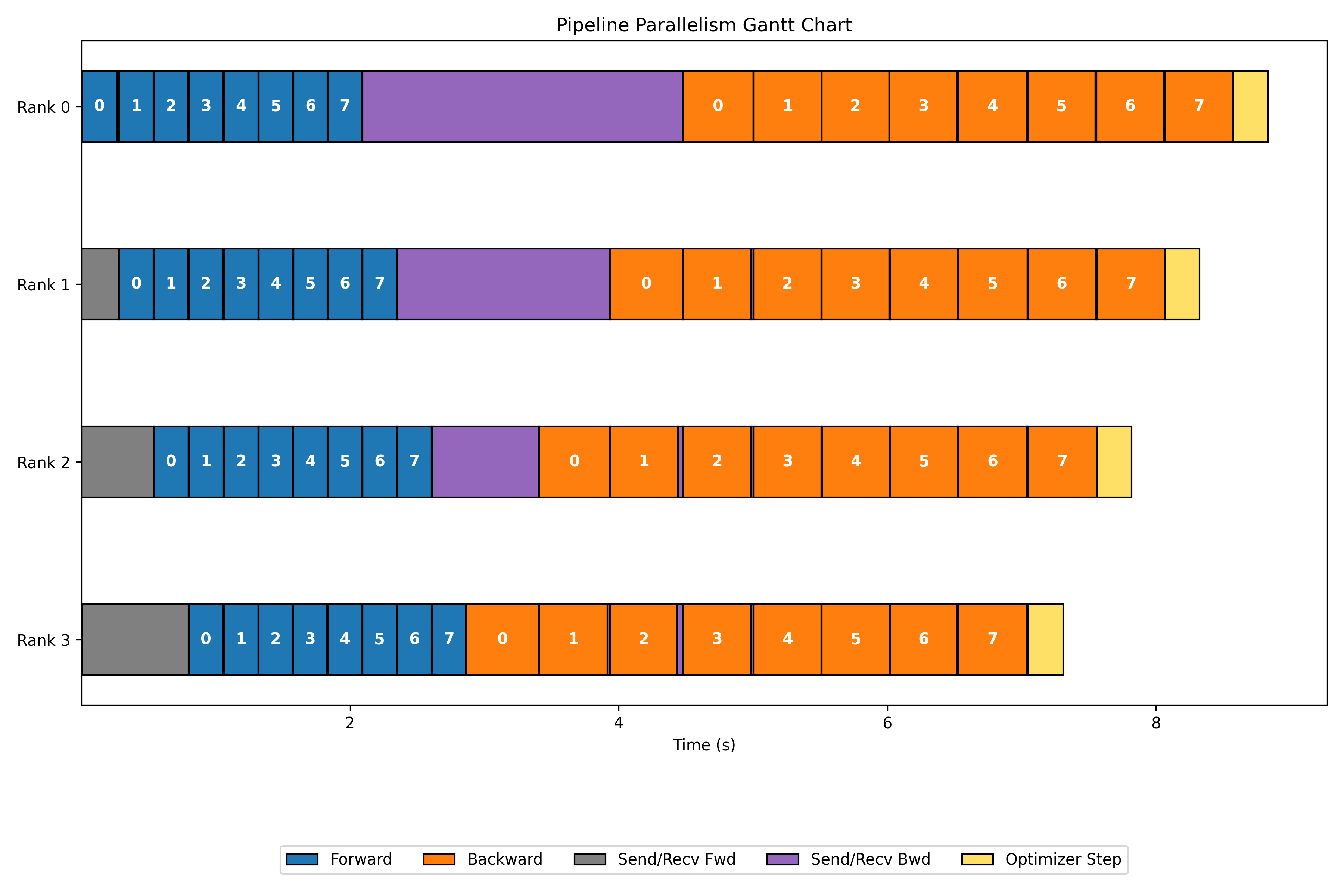
Gantt Chart
Executing the code results in the following Gantt chart, providing a visual representation of AFAB.
 </img>
1F1B: One Forward, One Backward
To run this example, launch the following command
torchrun --nproc_per_node=3 train_1f1b.py --grad_acc_steps 2 --pseudo_computation_time 0.5
The goal is to initiate the backward pass as soon as it becomes feasible. This means that immediately after completing the forward pass of a microbatch in the last layer, the backward pass should be computed and sent back.
Implementing these types of schedules can be complex, but most of them follow a similar three-stage pattern:
- Warmup phase: Each rank performs a forward pass and sends the output to the next rank.
- Steady phase: Each rank performs both forward and backward passes, sending results to the respective ranks as they become available.
- Cooldown phase: After all forward computations are complete (at the end of a batch, when microbatches are exhausted, or before the optimizer steps), each rank completes the backward computations and sends gradients to the previous rank.
Note: While 1F1B does not decrease idle time, it significantly reduces memory usage. This is because intermediate activations do not need to be retained for long – gradients are computed and consumed immediately.
Warmup Phase
This phase is exactly same as the All Forward phase in AFAB involving one-way communication of the forward computations. As a result, I omit the code for this phase here.
Steady Phase
Once the pipeline is fully loaded with microbatches, we enter the steady state. Each stage alternates between receiving forward and backward data, keeping both directions of the pipeline busy:
-
Each stage receives:
-
A new forward microbatch from the previous rank, and
-
A backward gradient from the next rank.
-
-
It then:
-
Executes the forward pass for the incoming microbatch.
-
Executes the backward pass for the oldest stored microbatch.
-
-
Finally, it:
-
Sends the computed gradient to the previous rank, and
-
Receives the next microbatch for forward processing.
-
This pipelined alternation helps maximize device utilization while keeping memory footprint low.
    print(f"[rank {pp_rank}] Steady state...\n")
    if num_microbatches_remaining > 0:
        input_tensor = pipeline_communicate(operation='recv_fwd', pp_rank=pp_rank, pp_world_size=pp_world_size, tensor_shape=tensor_shape)

    for i in range(num_microbatches_remaining):
        step_idx = num_warmup_microbatches + i
        # One forward step: process new input
        if input_tensor is None:
            input_tensor, _ = next(dataloader)
        output_tensor = model.forward(input_tensor)

        if pp_rank == pp_world_size - 1:
            _, target_tensor = next(dataloader)
            output_tensor = F.mse_loss(output_tensor, target_tensor, reduction='mean')
            loss += output_tensor.item() / grad_acc_steps

        input_tensors.append(input_tensor)
        output_tensors.append(output_tensor)

        # Bidirectional communication: send forward output, receive backward gradient (for the oldest microbatch)
        output_tensor_grad = bidirectional_pipeline_communicate(
            operation='send_fwd_recv_bwd', send_tensor=output_tensor, recv_tensor_shape=tensor_shape,
            pp_rank=pp_rank, pp_world_size=pp_world_size,
        )

        # One backward step: process oldest microbatch in queue
        input_tensor, output_tensor = input_tensors.pop(0), output_tensors.pop(0)
        input_tensor_grad = model.backward(input_tensor, output_tensor, output_tensor_grad)

        # Prepare for next iteration: send/receive as needed
        # Bidirectional communication: send backward output, receive input for the next forward step
        if i == num_microbatches_remaining - 1:
            input_tensor = None
            pipeline_communicate(
                operation='send_bwd', pp_rank=pp_rank, pp_world_size=pp_world_size, tensor=input_tensor_grad
            )
        else:
            input_tensor = bidirectional_pipeline_communicate(
                'send_bwd_recv_fwd', pp_rank=pp_rank, pp_world_size=pp_world_size,
                send_tensor=input_tensor_grad, recv_tensor_shape=tensor_shape
            )
Cooldown Phase
This phase is exactly same as the All Backward phase in AFAB involving one-way communication of the backward computations. As a result, I omit the code for this phase here.
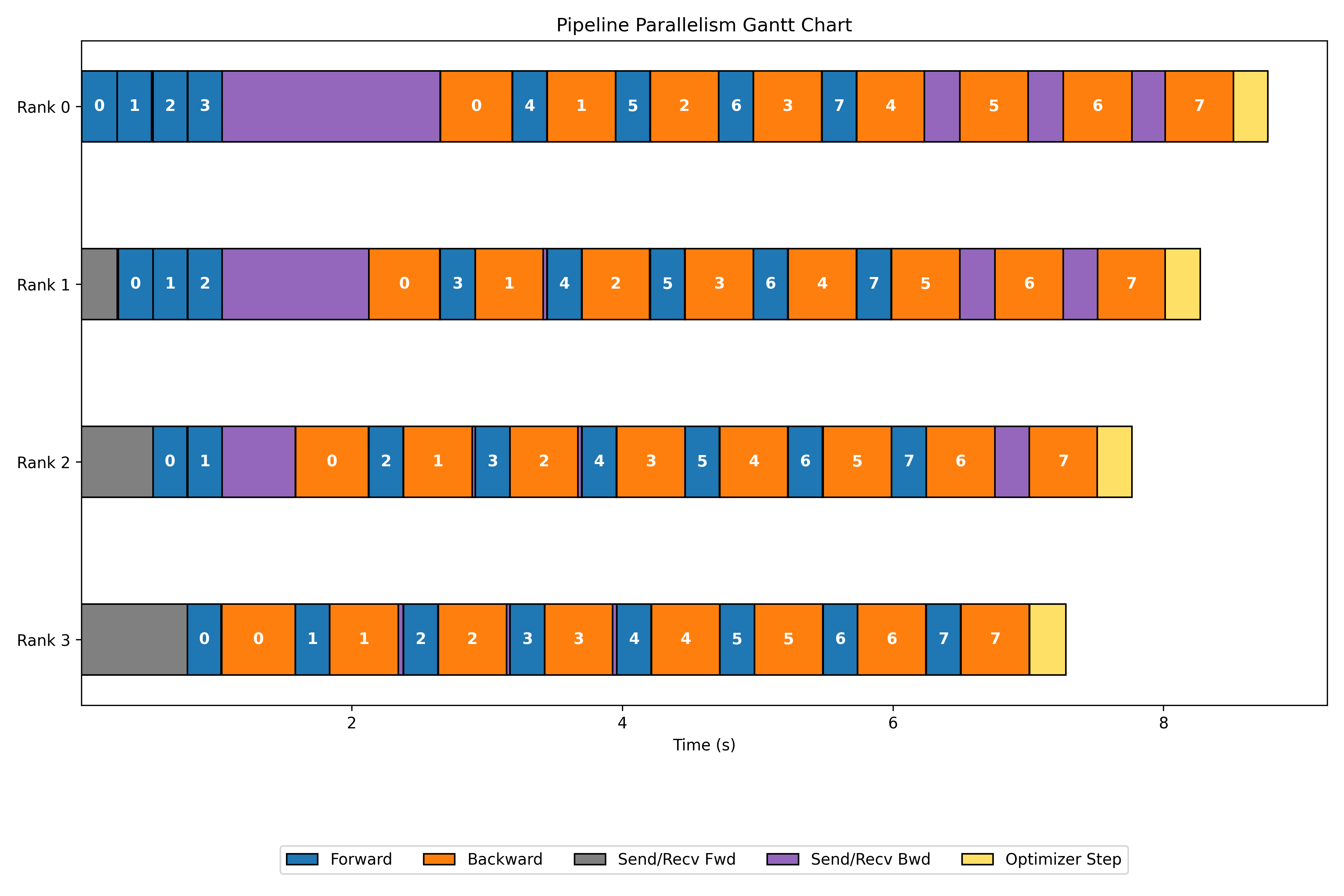
Gantt Chart
Executing the code generates the Gantt chart below, providing a visual representation of 1F1B.
 </img>
Other schedules
When analyzing the pipeline bubble, I focus on the last GPU to measure its idle time—specifically:
- The time spent waiting for forward input during the warm-up phase, and
- The time spent waiting for backward gradients to finish during the cooldown phase.
Two key factors influence the size of this bubble:
- The number of pipeline stages (\( p \)) — more workers generally mean longer idle periods at the ends.
- The forward (\( t_f \)) and backward (\( t_b \)) computation times.
Strategies to Reduce the Bubble.
-
Interleaving layers: Assigning non-contiguous layers (e.g., layer 1 and layer 5) reduces the effective \( t_f \) or \( t_b \) per stage and shrinks the bubble.
-
Prioritizing input gradients: By computing input gradients first (i.e., gradients w.r.t. activations) and postponing weight gradients, we can immediately pass gradients upstream. This overlap reduces the time each stage waits before initiating its own backward pass, essentially reducing \( t_b \)
I highly recommend exploring the Ultra Scale Playbook section on pipeline parallelism to understand this in more detail.