 Prateek Gupta
Understanding How Floating Point Representations Work
The impressive emergent capabilities of LLMs have largely been observed as a result of scaling them to massive sizes, sometimes with hundreds of billions of parameters (e.g., 470B or 600B). These models are enormous, with some requiring up to 500GB of disk space.
In response, the community has been working in two directions simultaneously:
- On one hand, there’s a push to compress the intelligence of large models into smaller, more efficient ones.
- On the other hand, there’s continued momentum toward even larger models, with trillions of parameters on the horizon.
One promising direction to enable this is to reduce the precision used in representing model parameters. Traditionally, neural networks have been trained using 32-bit floating point numbers (FP32). To scale models more efficiently, many are now trained using 16-bit precision (FP16 or BF16), and some even use mixed-precision formats, where certain parameters are stored in FP8 or lower.
This shift introduces the need for mixed-precision training, techniques that maintain reliable learning despite operating at reduced numerical precision. I explore that in detail in the next post.
But before going there, I want to revisit a more fundamental question: What is floating point representation, really?
It’s easy to forget that machines don’t reason in a continuous domain. Their numbers are actually discrete. So in this post, I want to give a hands-on exploration of floating point formats, to better understand and appreciate how numbers are actually represented inside machines.
How computers represent numbers?
In computers, all data is represented as a sequence of bits – each being either a 0 or a 1. Specifically, numbers are represented by a standardized format of 0s and 1s. For example, unsigned integers are represented by a sequence of 8 bits (also known as uint8). The standard python representation for decimal numbers uses 64 bits or 8 bytes (float64).
import sys
import numpy as np
import torch

print("Standard python float representation:")
a = 1.232
print("Type of a:", type(a))
print("Size of a (in bytes):", sys.getsizeof(a))
print("Extra overhead (bytes):", sys.getsizeof(a) - 8)
Standard python float representation:
Type of a: <class 'float'>
Size of a (in bytes): 24
Extra overhead (bytes): 16
Note: even though the representation of a float consumes 64 bits (8 bytes), it takes about 24 bytes in standard Python to store this number. The extra memory is used for Python’s object system to store reference counts, type info, etc.
Let’s look at how does Numpy or PyTorch represent other lower precision formats in 32 bits or 16 bits.
print("NumPy float representation:")
b = np.float32(1.232)
print("  Type of b:", type(b))
print("  Size of b (in bytes):", sys.getsizeof(b))
print("  Number of bits:", b.nbytes * 8)
print("  Extra overhead (bytes):", sys.getsizeof(b) - 4)

c = np.float64(1.232)
print("\n")
print("NumPy double representation:")
print("Type of c:", type(c))
print("Size of c (in bytes):", sys.getsizeof(c))
print("Number of bits:", c.nbytes * 8)
print("Extra overhead (bytes):", sys.getsizeof(c) - 8)

print("\n")
print("PyTorch float32 representation:")
c = torch.tensor(1.232, dtype=torch.float32)
print("Type of c:", type(c))
print("Size of c (in bytes):", sys.getsizeof(c))
print("Number of bits:", c.numel() * 32)
print("Extra overhead (bytes):", sys.getsizeof(c) - 4)


print("\n")
print("PyTorch float16 representation:")
d = torch.tensor(1.232, dtype=torch.float16)
print("Type of d:", type(d))
print("Size of d (in bytes):", sys.getsizeof(d))
print("Number of bits:", d.numel() * 16)
print("Extra overhead (bytes):", sys.getsizeof(d) - 2)
NumPy float representation:
    Type of b: <class 'numpy.float32'>
    Size of b (in bytes): 28
    Number of bits: 32
    Extra overhead (bytes): 24


NumPy double representation:
    Type of c: <class 'numpy.float64'>
    Size of c (in bytes): 32
    Number of bits: 64
    Extra overhead (bytes): 24


PyTorch float32 representation:
    Type of c: <class 'torch.Tensor'>
    Size of c (in bytes): 80
    Number of bits: 32
    Extra overhead (bytes): 76


PyTorch float16 representation:
    Type of d: <class 'torch.Tensor'>
    Size of d (in bytes): 80
    Number of bits: 16
    Extra overhead (bytes): 78
The way we perform arithmetic, addition, subtraction, multiplication, and division, is conceptually different from how machines handle these operations. Machines operate at the level of bits, relying on bitwise manipulations to carry out even the simplest computations.
Each numeric representation (e.g., float32, float16, bfloat16) requires dedicated kernels, low-level routines optimized for performing arithmetic on that specific format. Libraries like NumPy and PyTorch support floating point arithmetic using representations smaller than 64 bits (e.g., float32, float16, bfloat16). These libraries also include optimizations that enable efficient computation on lower-precision formats, often by using additional memory to support alignment, buffering, or fused operations. As a result, we notice higher memory overhead than expected.
Illusion vs. Reality of Representation
Computers are discrete representation machines; they store and process information in finite, countable steps, typically as sequences of 1s and 0s. Any sense of continuity, such as representing real numbers, is ultimately an illusion in a digital computer. In reality, these values are always approximated using a finite number of bits.
For example, when we store a floating-point number, we are not storing the real number itself, but rather a discrete approximation of it, limited by the number of bits allocated for the representation.
Between any two representable numbers, there are infinitely many real values the computer cannot distinguish.
So while mathematical models may assume perfect continuity, all computations on a digital machine are fundamentally discrete. What appears continuous is simply a clever approximation that works well enough for most practical applications.
Let’s see this illusion in practice:
a = 0.1
print(f"{a: 0.64f}")
0.1000000000000000055511151231257827021181583404541015625000000000
This output reveals the true stored representation of 0.1—which, as you can see, is not exactly 0.1.
This discrepancy arises from the limitations of binary floating-point formats: many decimal fractions simply cannot be represented exactly in binary.
Note: This is usually not a problem, unless high precision is critical in your application.
But how can this limitation lead to surprising behavior?
Arithmetic operations are performed at the bitwise level. When performing calculations, computers rely on binary manipulations that may introduce small errors, especially after multiple operations.
Here’s an example:
print("Result of 0.3 - 0.2 == 0.1:", 0.3 - 0.2 == 0.1)
print("Representation of 0.3 - 0.2:", 0.3 - 0.2)
print(f"Representation of 0.1: {0.1: 0.64f}", 0.1)
Result of 0.3 - 0.2 == 0.1: False
Representation of 0.3 - 0.2: 0.09999999999999998
Representation of 0.1: 0.1000000000000000055511151231257827021181583404541015625000000000 0.1
Although mathematically 0.3 - 0.2 should equal 0.1, the result is just slightly off, causing the equality check to return False.
Note: When comparing floating-point numbers, you should avoid exact equality checks. Instead, use an approximate comparison, checking whether the numbers are “close enough” within a small tolerance.
np.is_closedoes exactly that.
How are numbers represented in floating point?
A floating-point number is represented using three distinct components:
- Sign (S): A single bit indicating whether the number is positive or negative.
- Exponent (E): A set of bits that determines the number’s scale or magnitude.
- Mantissa (M) or Significand: A set of bits that defines the number’s precision or fractional part.
To make this concrete, let’s use a hypothetical 8-bit format for our examples: S EEE MMMM, which has 1 sign bit, 3 exponent bits, and 4 mantissa bits.
The Conversion Formula
We’ll stick to the widely adopted IEEE 754 standard, which ensures that floating-point representation and arithmetic are consistent across different machines. The value of a normal floating-point number (we’ll cover subnormal numbers in the next section) is calculated using a formula that closely resembles scientific notation:
\[ \text{Value} = (-1)^S \times (1.M)_2 \times 2^{(E - \text{bias})} \]
Let’s break this down:
- \( (-1)^S \): The sign bit
Sdetermines the sign.S=0for positive,S=1for negative. - \( (1.M)_2 \): This is the significand. It encodes the precision (the significant digits of the number). For normal numbers, there is an implicit leading
1followed by the mantissa bitsM. For subnormals (see below), there is no leading1, i.e., it is represented as \( (0.M)_2 \). The subscript2indicates this is a binary representation. - \( 2^{(E - \text{bias})} \): This is the scale factor.
Eis the decimal value of the exponent bits, andbiasis a predefined constant.
Note: The expression above mirrors scientific notation in base 10, for example:
\[ -1 \times 3.539820 \times 10^{-9} \]
The floating-point version just uses base 2 instead of base 10.
The Sign Bit (S)
This is the most straightforward part. It’s the first bit: 0 for a positive number, 1 for a negative number.
The Scale bits: Exponent (E) and Bias
The exponent bits allow us to represent numbers across a vast range, from very small to very large. To represent both positive and negative exponents (e.g., \( 2^{10} \) and \( 2^{-10} \)) without needing a separate sign bit for the exponent, the standard uses a biased representation.
The actual exponent is calculated as E_decimal - bias, where E_decimal is the unsigned integer value of the exponent bits. The bias is a fixed constant calculated as:
\[ \text{bias} = 2^{\text{exponent_bits}-1} - 1 \]
For our 3-bit exponent example, the bias = 2^(3-1) - 1 = 3. This allows the exponent range to be centered around zero.
Thus, we represent non-negative numbers smaller than 1 whenever \( E < bias \).
The Precision bits: Mantissa (M)
Once the scale is determined by the exponent bits, the mantissa (or significand) allows us to represent numbers that are \( \epsilon \)-close to that scale. The mantissa provides this fine-grained precision around the chosen magnitude.
Precision of a format can be understood as the smallest step size between two adjacent representable numbers at a given scale. Higher precision means that the distance between two neighboring representable numbers is smaller. In other words, the format can represent values that are more finely spaced, allowing for more accurate approximations of real numbers.
A binary number like \( (1.m_1m_2m_3m_4)_2 \) is converted to a decimal fraction as:
\[ (1.m_1m_2m_3m_4)_2 = 1 \times 2^0 + m_1 \times 2^{-1} + m_2 \times 2^{-2} + m_3 \times 2^{-3} + m_4 \times 2^{-4} \]
Putting it all together, the full formula for a normal number expands to:
\[ \text{Value} = (-1)^S \times \left(1 + \sum_{i=1}^{\text{num_mantissa_bits}} m_i \cdot 2^{-i}\right) \times 2^{(E - \text{bias})} \]
To find out how to view the binary representation behind floating point numbers, please see the Appendix.
Normal vs Subnormal Numbers
IEEE 754 standard distinguishes between two types of floating-point numbers:
Normal Numbers
- When exponent is not all
0s or all1s. - These numbers are interpreted as: \( (-1)^S \times (1.M)_2 \times 2^{(E - \text{bias})} \)
- The leading
1.is implicit, allowing us to store one extra bit of precision without specifying it.
Subnormal Numbers
- When exponent bits are all 0s.
- It is interpreted as: \( (-1)^S \times (0.M)_2 \times 2^{(1 - \text{bias})} \)
- The leading 1. is not assumed. Instead, the standard uses a leading
0instead.
These numbers are smaller than the smallest normal, providing a gradual underflow instead of jumping straight to zero.
Visualizing How Floating Point Numbers Sit on the Real Number Line
Let’s explore where key floating-point numbers lie on the number line, particularly around zero, where subnormals come into play.
- Smallest positive normal number is when
E=1andM=0: \( 2^{1-bias} \) -
Largest positive subnormal number is when
E=0andM=2^m -1, i.e., all1s: \( 2^{1-bias} \times (0.M)_2 = 2^{1-bias} \times (1 - 2^{-m}) \). For example, withm=3, \[ (0.111)_2 = \frac{1}{2} + \frac{1}{2^2} + \frac{1}{2^3} = 1 - 2^3 \] - Smallest positive subnormal number (excluding +0) is when
E=0andM=1: \( 2^{1-bias} \times 2^{-m} = 2^{1-bias-m}\). For example, withm=3, \[ (0.001)_2 = 0 + 0 + \frac{1}{2^3} \]
Even Spacing Between Two Scales
We can factor a binary fraction like \( 0.m_1m_2m_3 \) as
\[ m_1 \times 2^{-1} + m_2 \times 2^{-2} + m_3 \times 2^{-3} = 2^{-3} \times (m_1 \times 2^2 + m_2 \times 2^1 + m_3 \times 2^0) = 2^{-3} \times (M)_{10} \]
Given a fixed exponent, the mantissa bits define how finely we can place values between two powers of two. That is, they determine the granular spacing of representable numbers.
Thus, the spacing between consecutive floating-point numbers at a given exponent is: \[ 2^{exp-bias} \times 2^{-m}, \]
Computing the difference between the smallest normal number and the largest subnormal number, we obtain the step size of \( 2^{1-bias-m} \), where \( m \) is the number of mantissa bits. By design, the difference between the smallest positive subnormal number and \( 0 \) is also \( 2^{1-bias-m} \). This consistent spacing ensures that subnormals provide a smooth and uniform transition from the smallest normal number down to zero, preventing a sudden gap in the number line.
Without subnormals, there would be a sudden gap between the smallest normal number and zero, creating a significant gap in the number line.
Subnormals elegantly solve this problem by filling the gap between the smallest normal number and zero. They maintain the same step size of \( 2^{1-bias-m} \).
Let’s illustrate this scale dependent precision and uniform transition to 0 this via code. Here, I have used FP8 E4M3 format, which uses S EEEE MMM format for representation, i.e., 1 sign-bit, 4 exponent bits, and 3 mantissa bits.
import numpy as np
import matplotlib.pyplot as plt


# For FP8 E4M3 format:
# - 1 bit for sign
# - 4 bits for exponent (bias = 2^3 - 1 = 7)
# - 3 bits for mantissa

numbers = []
# We'll focus on positive numbers (sign bit = 0)

# Handle subnormal numbers (exp = 0)
for mant in range(1, 8):  # Skip mant=0 as it represents zero
    # For subnormals: 0.mantissa * 2^(1-bias)
    value = (mant/8) * 2**(1-7)  # 1-bias = 1-7 = -6
    numbers.append(value)

# Add normal numbers close to subnormals (exp = 1)
for mant in range(8):  # Include all mantissa combinations
    # For normals: 1.mantissa * 2^(exp-bias)
    value = (1 + mant/8) * 2**(1-7)  # exp=1, bias=7
    numbers.append(value)

# Handle normal numbers
for exp in range(7, 11):  # exponents from 7 to 10
    # For each exponent, generate all possible mantissa combinations
    for mant in range(8):  # 3 bits = 8 combinations
        # Calculate the value: 1.mantissa * 2^(exp-bias)
        value = (1 + mant/8) * 2**(exp-7)
        numbers.append(value)

plt.figure(figsize=(15, 2))
plt.scatter(numbers, [0]*len(numbers), s=100, alpha=0.6)
plt.xlim(0.9, 8.1)
plt.ylim(-0.1, 0.1)
plt.grid(True, axis='x')
plt.title('FP8 E4M3 Numbers between 1 and 8')
plt.xlabel('Value')
plt.xticks([1, 2, 4, 8])
plt.yticks([])  # Remove y-axis ticks
plt.show()

# Plot numbers between smallest normal and largest subnormal
plt.figure(figsize=(15, 2))
plt.scatter(numbers, [0]*len(numbers), s=100, alpha=0.6)

# Find smallest normal and largest subnormal
smallest_normal = 2**(1-7)
penultimate_normal = 2**(1-7) * (1 + 7/8)
largest_subnormal = 2**(1-7) * 7/8

# Add vertical lines to mark these values
plt.axvline(x=smallest_normal, color='r', linestyle='--', alpha=0.5, label=f'Smallest Normal: {smallest_normal:.6f}')
plt.axvline(x=largest_subnormal, color='g', linestyle='--', alpha=0.5, label=f'Largest Subnormal: {largest_subnormal:.6f}')

plt.xlim(0, penultimate_normal*1.1)  # Show region around transition
plt.ylim(-0.1, 0.1)
plt.grid(True, axis='x')
plt.title('FP8 E4M3 Numbers: Transition from Normal to Subnormal')
plt.xlabel('Value')
plt.yticks([])  # Remove y-axis ticks
plt.legend()
plt.show()
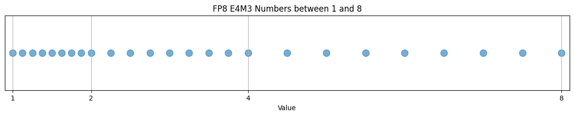
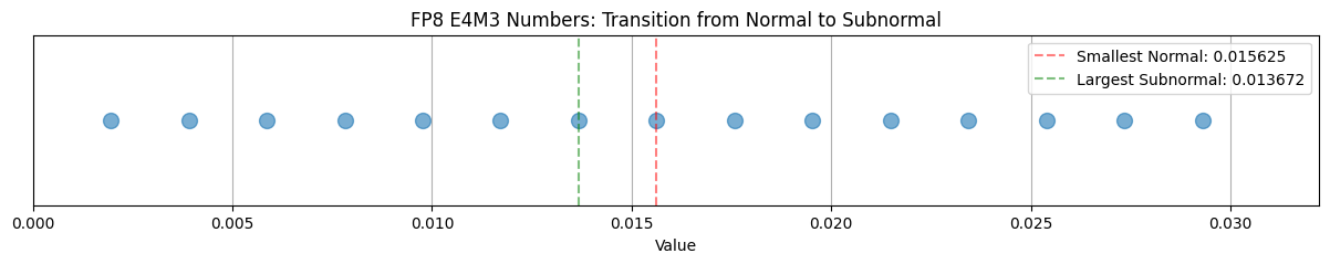
We clearly see that the precision (step sizes) decreases with the scale. In addition, we can also spot the smooth and uniform transition of representable numbers to \( 0 \).
Special Cases: Zero, Infinity, and Subnormals
The IEEE 754 standard reserves certain bit patterns for special values. The value of the exponent bits is key to distinguishing these cases.
| Exponent Bits | Mantissa Bits | Represents |
|---|---|---|
| All 0s | All 0s | Zero (+0 or -0, depending on the sign bit) |
| All 0s | Non-zero | Subnormal Numbers. Represented as \( (-1)^S \times (0.M)_2 \times 2^{1 - \text{bias}} \) |
| All 1s | All 0s | Infinity (+inf or -inf) |
| All 1s | Non-zero | NaN (Not a Number) |
Unequal Spacing: A Concrete Example with FP8 E4M3
Thanks to Puneet Dokania for providing feedback. This detailed walkthrough should help anyone trying to grasp FP representation.
Let’s work through a concrete example to understand how step sizes vary across different scales in floating-point representation. We’ll use the FP8 E4M3 format, which has 1 sign bit, 4 exponent bits, and 3 mantissa bits.
Understanding the format:
- Exponent bits (EEEE): 4 bits with bias = 2³ - 1 = 7
- Mantissa bits (MMM): 3 bits, giving us 8 possible values (0 through 7)
- Largest exponent: EEEE = 1110₂ = 14 (1111₂ is reserved for NaN/infinity)
Step size calculation: The step size at any given exponent is determined by the contribution of the least significant mantissa bit: \[ \text{Step size} = 2^{(\text{exponent} - \text{bias})} \times 2^{-\text{num_mantissa_bits}} \]
For FP8 E4M3, this becomes: \[ \text{Step size} = 2^{(\text{exponent} - 7)} \times 2^{-3} = 2^{(\text{exponent} - 10)} \]
Let’s trace through the mantissa arrangements: With 3 mantissa bits, we have 8 possible combinations (000₂ through 111₂):
| Binary | Fraction | Value |
|---|---|---|
| 000₂ | 0/8 | 0.000 |
| 001₂ | 1/8 | 0.125 |
| 010₂ | 2/8 | 0.250 |
| 011₂ | 3/8 | 0.375 |
| 100₂ | 4/8 | 0.500 |
| 101₂ | 5/8 | 0.625 |
| 110₂ | 6/8 | 0.750 |
| 111₂ | 7/8 | 0.875 |
Thus, in FP8 E4M3, at any given exponent, there are exactly 8 representable numbers, each separated by a step size of 2⁻³ = 0.125 times the scale factor.
Step sizes across the range:
-
Largest exponent (14): Step size = 2^(14-10) = 2⁴ = 16 The representable numbers at this scale are: \[ 2^{14} \times (1.000, 1.125, 1.250, 1.375, 1.500, 1.625, 1.750, 1.875) \] Which gives us: 16384, 18432, 20480, 22528, 24576, 26624, 28672, 30720
Notice that each number is 16,384 units apart - a massive step size!
-
Smallest exponent (1): Step size = 2^(1-10) = 2⁻⁹ ≈ 0.00195 The representable numbers at this scale are: \[ 2^{-6} \times (1.000, 1.125, 1.250, 1.375, 1.500, 1.625, 1.750, 1.875) \] Which gives us: 0.015625, 0.017578, 0.019531, 0.021484, 0.023438, 0.025391, 0.027344, 0.029297
Here each number is only 0.001953 units apart - much finer precision!
-
Subnormal numbers (exponent 0): Step size = 2^(1-7-3) = 2⁻⁹ ≈ 0.00195 The representable numbers are: \[ 2^{-6} \times (0.125, 0.250, 0.375, 0.500, 0.625, 0.750, 0.875) \] Which gives us: 0.001953, 0.003906, 0.005859, 0.007813, 0.009766, 0.011719, 0.013672
Even finer spacing near zero!
This demonstrates the unequal spacing characteristic of floating-point: numbers near zero are much more densely packed than large numbers. The step size grows exponentially with the magnitude, which is why we can represent both very small and very large numbers with the same number of bits.
Arithmetic with Subnormals
Operations involving subnormals often require special handling in hardware: When performing arithmetic operations with subnormal numbers, the process typically involves three steps:
- Normalize the subnormal numbers to regular floating-point form
- Execute the arithmetic operation
- Denormalize the result back to subnormal form if needed
This additional processing introduces both latency and energy overhead. To mitigate these performance impacts, many systems, particularly in machine learning applications, implement a “flush-to-zero” (FTZ) mode. In FTZ mode, any subnormal number is automatically converted to zero before the operation begins.
NVIDIA’s CUDA platform, however, offers efficient support for FMA (Fused Multiply-Add) operations on subnormal numbers. Other operations on subnormals might require specialized kernels and run slower. For more details on NVIDIA’s approach to mixed precision and FMA operations, you can refer to their blog post on mixed precision programming.
One thing to keep in mind when using reduced precision is that because the normalized range of FP16 is smaller, the probability of generating subnormal numbers (also known as denormals) increases. Therefore it’s important that NVIDIA GPUs implement FMA operations on subnormal numbers with full performance. Some processors do not, and performance can suffer. (Note: you may still see benefits from enabling “flush to zero”. See the post “CUDA Pro Tip: Flush Denormals with Confidence”.) – Mixed Precision Programming Blog, NVIDIA
Precision bias towards 0
One interesting aspect of IEEE 754 floating-point representation is the asymmetric distribution of representable numbers around zero.
The format allocate significantly more bit patterns to values closer to zero than to larger numbers.
This is because the exponent field in IEE 754 format is centered around a bias - expeonents below the bias respresent small magnitudes (less than 1) and above the bias represent larger values (greater than 1).
This design choice becomes particularly evident in deep learning. During model training, a significant portion of the computation involves values much smaller than 1. This is visually confirmed by Figure 3 from Mixed Precision Training by Narang et al.
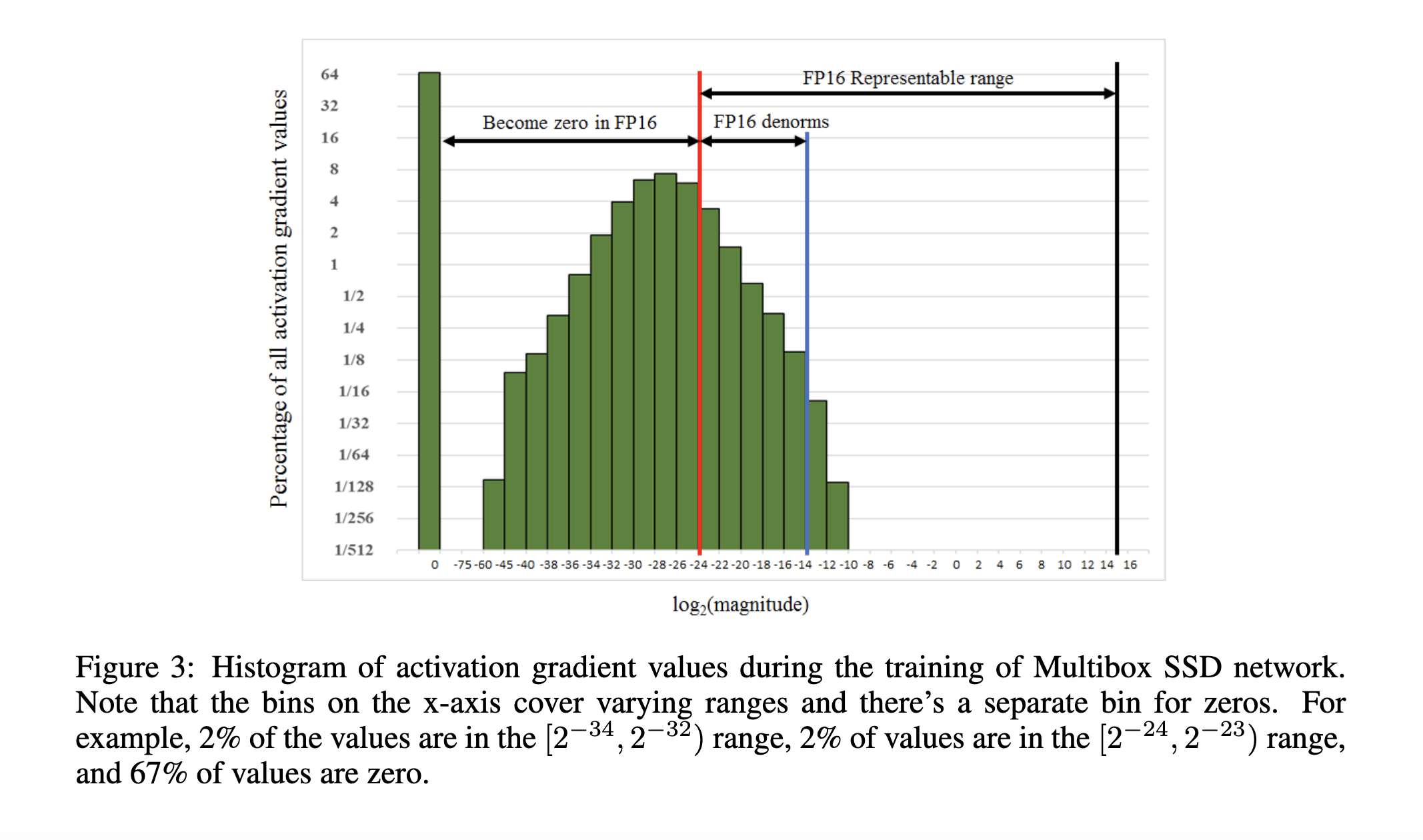
As the figure shows, the lower half of FP16’s range is densely populated with values. The upper half—which represents much larger numbers—is rarely used during training. While the original paper introduces this observation in the context of loss scaling (which we’ll explore in the next post), it also highlights a broader point:
Floating-point formats are intentionally designed to offer higher resolution near zero, where most computations actually happen.
This precision bias benefits not only deep learning but also many other fields, like scientific computing and signal processing, where small values dominate and accuracy in the low range is essential.
What is Overflow and Underflow?
Every floating-point format has a limited representable range. For example, in the float32 (IEEE 754 single precision) format, the range of positive values is approximately:
\[ [1.4 \times 10^{-45},\ 3.4 \times 10^{38}] \]
As we saw earlier, not all real numbers within this range can be represented exactly—e.g., 0.1 is only approximated.
But there are also numbers outside this range that cannot be represented at all:
-
Overflow occurs when a value exceeds the maximum representable value. The result is typically stored as
inf(infinity), or triggers an error depending on the system. -
Underflow occurs when a value is smaller (in magnitude) than the smallest representable positive number. These values are either:
- Rounded to zero, or
- Represented as subnormals if the format supports it (as we discussed earlier).
Underflow doesn’t usually cause crashes, but overflow often does, especially if not handled gracefully.
What are different types of representation?
Standard representations are FP64, FP32, FP16, BF16 (Brain-Float), FP8 E4M3, FP8 E5M2.
These representations differ in their total number of bits, the bits for exponent, and the bits for mantissa. They all have one dedicated bit for sign at the beginning.
| Format | Total Bits | Exponent Bits | Mantissa Bits |
|---|---|---|---|
| FP64 | 64 | 11 | 52 |
| FP32 | 32 | 8 | 23 |
| FP16 | 16 | 5 | 10 |
| BF16 | 16 | 8 | 7 |
| FP8 E4M3 | 8 | 4 | 3 |
| FP8 E5M2 | 8 | 5 | 2 |
For a better understanding of differences between FP16 and BF16, read here.
Let’s look at their characteristics :
# Code from: https://medium.com/data-science/pytorch-native-fp8-fedc06f1c9f7
import torch
from tabulate import tabulate

f32_type = torch.float32
f16_type = torch.float16
bf16_type = torch.bfloat16
fp8_e4m3_type = torch.float8_e4m3fn

table = []
for dtype in [f32_type, f16_type, bf16_type, fp8_e4m3_type]:
    info = torch.finfo(dtype) # See here for finfo: https://docs.pytorch.org/docs/stable/type_info.html
    table.append([
        info.dtype,
        info.bits,
        info.max,
        info.min,
        info.smallest_normal,
        info.eps,
    ])


headers = ["Format", "Total Bits", "Max", "Min", "Smallest Normal", "Eps"] #, "Max Exp", "Min Exp", "Min Subnormal", "Max Subnormal"]
print(tabulate(table, headers=headers))
Format           Total Bits              Max               Min    Smallest Normal          Eps
-------------  ------------  ---------------  ----------------  -----------------  -----------
float32                  32      3.40282e+38      -3.40282e+38        1.17549e-38  1.19209e-07
float16                  16  65504            -65504                  6.10352e-05  0.000976562
bfloat16                 16      3.38953e+38      -3.38953e+38        1.17549e-38  0.0078125
float8_e4m3fn             8    448              -448                  0.015625     0.125
We’ve already seen that more mantissa bits lead to finer granularity, i.e., a smaller step size between two representable numbers in a given format. The Eps values in the table above represent the smallest distinguishable difference from 1.0—mathematically, this is the contribution from the Least Significant Bit (LSB) or the last mantissa bit and equals \( 2^{-m} \), where \( m \) is the number of mantissa bits.
In simple terms, if a number smaller than
Epsis added to 1.0, the result will still be 1.0 due to rounding.
Naturally, low-precision formats like FP8, which have fewer mantissa bits, suffer from coarse granularity. This can lead to numerical instability, especially when representing small gradients or performing subtle updates during training.
To mitigate these issues, special training frameworks are required that can compensate for the reduced precision. This is what we will explore in the next post: Understanding Mixed-Precision Training Techniques.
Appendix
How to check binary representation behind the floating point numbers?
This is a neat trick that I recently learned while debugging mixed-precision arithmetic. We can use PyTorch’s .view() method to perform a “reinterpret cast”, a technique systems programmers often use in C++.
Most PyTorch users only use view() to change the shape of a tensor (similar to reshape). However, it has a secondary “superpower”: it can reinterpret the datatype of the data in memory without changing the actual bits.
This allows us to peek under the hood and see exactly how a floating-point number is stored in IEEE 754 format.
1. The PyTorch Way: Using .view()
To see the bits of a float32, we view it as an int32. The memory stays the same, but PyTorch now treats those 32 bits as an integer, which we can easily print in binary. It stops caring about what the bits “mean” mathematically (exponent, mantissa, sign). In contrast, if you tried to use .to(torch.int32), PyTorch would perform a mathematical conversion, rounding 0.01 down to 0.
import torch

# Create a float32 tensor
val = 0.01
s = torch.tensor(val, dtype=torch.float32)

# "Reinterpret" the bits as a 32-bit integer
# We use .item() to get the Python integer out, then format it.
# :032b means "32 bits wide, padded with zeros"
binary_str = f"{s.view(torch.int32).item():032b}"

print(f"Decimal: {val}")
print(f"Binary:  {binary_str}")

# Output:
# Decimal: 0.01
# Binary:  00111100001000111101011100001010
This trick works for other precisions too, which is essential for comparing float16 vs bfloat16. Just remember to mask the output for 16-bit types so Python doesn’t print extra sign bits:
# For float16 (Half Precision), view as int16
s_fp16 = torch.tensor(0.01, dtype=torch.float16)
print(f"FP16: {s_fp16.view(torch.int16).item() & 0xffff:016b}")
2. The Python Way: Using struct
What if you aren’t using PyTorch? Standard Python float objects are actually 64-bit doubles (similar to C’s double). Python doesn’t have a built-in view method or bin() for floats, so we have to use the struct module to manipulate the bytes directly.