 Prateek Gupta
Understanding Mixed-Precision Training
Several clever innovations have made it feasible to train large language models (LLM) with hundreds of billions of parameters, some even reaching 600B. However, there’s also increasing pressure to make them efficient to train and use for inference.
One area that has proven especially impactful is mixed-precision training, a technique where certain model parameters are stored and computed in lower precision formats (like FP8), while others remain in higher precision formats (like FP16 or FP32). For example, the FP8 format is used in certain modules of DeepSeek models
This led me to wonder: How is it even possible to train something as intelligent as a large language model using such low-precision numbers? What does it mean to “compress” intelligence into fewer bits?
To explore this, I first dove into the fundamentals of floating point representation. In this post, I cover the techniques that make mixed-precision training possible.
Why Use Mixed Precision?
When it comes to training LLMs, memory becomes a major bottleneck. There are typically five components that consume significant memory:
- Weights: The model’s parameters.
- Gradients: Computed during backpropagation for each parameter.
- Optimizer states: For optimizers like Adam, this includes the first and second moments (mean and variance) for each parameter.
- Activations: Intermediate hidden states stored during the forward pass to compute gradients later.
To reduce memory pressure, mixed precision training has become a widely adopted strategy. There are three compelling reasons to adopt it:
- Matrix multiplications and other operations execute significantly faster in lower precision formats
- When training across multiple GPUs, lower precision means fewer bytes to transfer, leading to faster data communication
- Reduced precision parameters require less memory, allowing for larger models or batch sizes
Quantization (converting high precision to low precision) is used in both training and inference. However, this post will focus specifically on mixed precision during the training phase, not inference.
Origins of Mixed-Precision Training
The original Mixed Precision Traininginf.
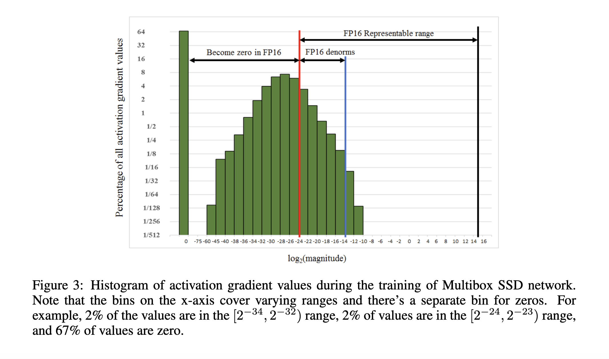
Figure 3 of the paper illustrates the distribution of gradient values, revealing that many gradient values fall below the representable range of FP16 format.
Since the paper’s publication, significant progress has been made in making mixed precision training practical. For instance, Deepseek-V3 recently trained their LLMs using FP8 format for certain operations.
What to Store in Lower Precision Format?
Choosing which components of a model to store in lower versus higher precision depends on several practical considerations:
- Memory Usage: Parameters or intermediate tensors that consume a large amount of memory, such as activations, are often good candidates for lower precision storage.
- Byte Transfer: When data transfer becomes a bottleneck, using lower precision formats helps by reducing the volume of bytes transmitted.
- Compute Density: For operations dominated by matrix multiplications (e.g., attention or MLPs), using lower precision inputs with higher precision accumulation can strike a balance between efficiency and accuracy.
Ultimately, the decision of which components require higher precision is empirical and model-specific.
As an example, Deepseek outlines their heuristics in section 3.3.1 of their technical report
Despite the efficiency advantage of the FP8 format, certain operators still require a higher precision due to their sensitivity to low-precision computations. Besides, some low-cost operators can also utilize a higher precision with a negligible overhead to the overall training cost. For this reason, after careful investigations, we maintain the original precision (e.g., BF16 or FP32) for the following components: the embedding module, the output head, MoE gating modules, normalization operators, and attention operators. These targeted retentions of high precision ensure stable training dynamics for DeepSeek-V3.
Note: Each new numerical format typically requires custom low-level code to handle its specific operations and optimizations. Efficient mixed-precision arithmetic operations require specialized hardware and software implementations.
Components of Mixed-Precision Training
From all my readings, I’ve learnt that there are four main concepts that enable reliable mixed-precision training:
In all my readings, I have decoded four basic concepts that are needed to enable MPT. These are
- Maintain a higher-precision copy of model weights. Even if weights are used in lower precision during computation, an FP32 (or higher) master copy is maintained to preserve numerical stability during updates.
- Use loss scaling to prevent gradient underflow. Scaling up the loss before backpropagation ensures that gradients remain above the minimum representable value in lower precision formats like FP16 or FP8.
- Perform computations in lower precision, but accumulate in higher precision. Matrix multiplications and other operations use low precision for inputs, but the results are accumulated in higher precision buffers (e.g., FP32) to reduce rounding errors.
- Carefully cast from higher to lower precision with input-aware strategies. When converting tensors to lower precision, the distribution of the input must be considered to avoid overflows and information loss.
Master Weights
Master weights are high-precision copies of model parameters (typically stored in FP32). During training, while the forward and backward passes operate on lowrer-precision weights (e.g., FP16 or BF16), all gradient updates area applied to the master weights. That is, the lower-precision gradients are accumulated into the high-precision master weights to preserve numerical accuracy. After each optimizer step, these master weights are cast back to lower precision (e.g., FP16 or FP8) for use in the next forward and backward passes.
Recall from our previous discussion on floating-point representation: the number of mantissa bits determines the precision, i.e., the step size between two representable numbers at a given scale. Specifically, it exhbits coarser step sizes (lower precision) at higher magnitudes (as shown in thenumber line plot).
This matters during training. Consider a case when a particular weight parameter \( W_i \) is large, e.g., around 5. If we represent this in lower formats like FP8, the representable numbers in FP8 around 5 have a coarser step size. This means that any update \( \Delta W_i \) that is less than the step size is as good as no update because it leaves the weight unchanged.
In a low-precision format, the magnitude of \( W_i \) might cause the fine-grained update \( \Delta W_i \) to be completely lost, i.e., the value doesn’t change at all. The lower precision simply lacks the granularity to represent such a small update at that scale.
Under the hood: Learning rate multiplication further reduces the magnitude of the weight update, increasing the risk of underflow in low-precision formats. To avoid this, the update is not written to a low-precision buffer. Instead, it is applied directly to the high-precision master weights, ensuring that small updates are not lost due to limited numerical resolution.
Loss Scaling
When training with FP16, gradients can become so small that they fall below the representable range of the format. To solve this, the Mixed Precision Training
The process has two key steps:
- Scale the loss before backward pass to avoid underflow.
- Unscale the gradients just before the optimizer step.
This approach maintains numerical stability while enabling efficient FP16 training.
Here’s how it looks in PyTorch:
import torch
LOSS_SCALE = 2**6

# Create a simple model
model = torch.nn.Sequential(
    torch.nn.Linear(10, 20),
    torch.nn.ReLU(),
    torch.nn.Linear(20, 5)
)

# Convert model to half precision
model = model.half() # FP16 format

# Create master weights in full precision
model_params = [p for p in model.parameters() if p.requires_grad]
master_params = [p.detach().clone().float() for p in model_params] # FP32 format

for p in master_params:
    p.requires_grad = True


# define optimizer on master weights
optimizer = torch.optim.SGD(master_params, lr=0.01)

optimizer.zero_grad()

# compute loss on dummy data
loss = torch.nn.MSELoss()(model(torch.randn(10)), torch.randn(5))

# compute gradients
loss.backward(LOSS_SCALE) # this will compute gradients on half precision model

# At the time of update, copy gradients from half precision model to master weights
for model, master in zip(model_params, master_params):
    master.grad.data.copy_(model.grad.data)


# scale down gradients by loss scale
if LOSS_SCALE is not None:
    for p in master_params:
        p.grad = p.grad / LOSS_SCALE

# W - lr * \Delta W
optimizer.step() # this will update master weights in full precision


# Cast the master params (FP32) to model params (FP16)
for model, master in zip(model_params, master_params):
    model.data.copy_(master.data)
Accumulation Precision
Many operations in MPT involve low-precision inputs (e.g., FP8 or GP16) that are accumulated in higher precision (e.g., FP16 or FP32). This requires specialized hardware and low-level optimizations to handle such operations efficiently.
Modern NVIDIA GPUs (starting with the Volta architecture like the V100) feature specialized tensor cores designed for matrix operations in various precision formats. In contrast, older GPUs relied solely on CUDA cores optimized for FP32 computations.
Matrix multiplication operations, which form the backbone of neural networks, involve numerous fused multiply-add operations. For instance, in a typical transformer architecture, the MLP layers process 4096-dimensional vectors, resulting in several thousands of such operations per layer.
Accumulating results in low-precision formats can significantly magnify numerical errors.
Empirical findings from DeepSeek indicate that accumulating FP8 products into FP16 buffers can already introduce up to 2% absolute error. If accumulation were performed in FP8 itself, the error would be much worse.
To mitigate this, compute-intensive operations are designed to accumulate in higher-precision registers, which are then cast down to lower precision after accumulation. In practice, PyTorch natively supports these operations for 16-bit formats (e.g., FP16, BF16). Support for 8-bit formats like FP8 is still experimental and evolving as of this writing.
from torch.cuda.amp import autocast

A = torch.randn(1024, 512, dtype=torch.float16)
B = torch.randn(512, 256, dtype=torch.float16)

with autocast(dtype=torch.float16):
    # the inputs will be in FP16 and the output will be in FP32 accumulation which will be cast down to FP16
    C = torch.matmul(A, B) # accumulation into FP32 registers

print(C.dtype)
torch.float16
Quantization
The term “quantization” comes up in three main contexts:
-
Pre-training (e.g., mixed-precision training): This is the focus of this post.
-
Quantization-Aware Training (QAT): This is a post-training method to adapt the pre-trained model to quantized weights. By simulating the effects of quantization during the post-training process, QAT helps the model adapt to the lower precision. It is often quite difficult due to non-differentiable operations like rounding to integers. Tricks like Straight-Through Estimators are used to pass the gradients through such operations. Read more about this here
. -
Post-Training Quantization (PTQ): There is no training involved. It shrinks the model by converting its weights from 32-bit floating-point numbers to smaller 8-bit or 4-bit integers. The results of integer arithmetic are dequantized for operations requiring higher precisions such as layernorm and softmax.
Quantization in Mixed-Precision Training
Let’s have a look at the MLP module in Deepseek-V3 Report
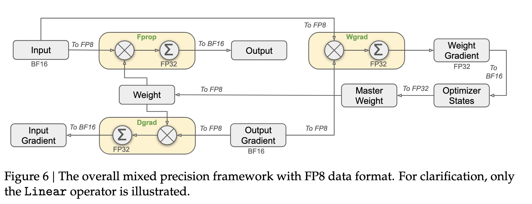
The image above shows the mixed-precision GEMM (Generalized Matrix Multiplication) operations for MLP module in the Deepseek-V3 architecture.
The yellow boxes correspond to matrix multiplication, where (X) is the matrix multiply and (\( \Sigma \)) is the accumulation operation in higher precision (FP32).
FProp is the forward propagation operation while Wgrad is the backpropagation operation to obtain \( \Delta W \), and the Dgrad is the backpropagation operation to obtain \( \Delta x \).
Everytime there is “To BF16” or “To FP8”, there is quantization taking place.
Thus, the inputs and weights are being quantized to FP8 format for matrix-multiply operations.
What does quantization involve technically?
In simple terms, quantization is converting inputs from higher precision to lower precision.
This can be done in three ways:
Naive or elementwise: Simply downcast by rounding the input to the nearest representatable value in the target format. For example, converting input from FP16 (which can represent large numbers) to FP8 E4M3 (which has a smaller range). This has serious limitations:
- Underflow: Very small values become zero
- Overflow: Values outside the representable range becomes
NaNorinf. - Precision loss: Fine-grained differences are lost.
Here is a simple code to illustrate such loss in precision:
import torch
from tabulate import tabulate

# Initialize random numbers in FP32 format
x = torch.randn(4, 1, dtype=torch.float32)
print("Original FP32 tensor:")
print(x)

# Downcast to FP16
x_bf16 = x.to(torch.bfloat16)

x_fp16 = x.to(torch.float16)

# Downcast to FP8 using torch's FP8 format
# Note: torch.float8_e4m3fn is available in newer PyTorch versions
try:
    x_fp8 = x.to(torch.float8_e4m3fn)
except AttributeError:
    # Fallback for older PyTorch versions
    print("torch.float8_e4m3fn not available, using FP16 as approximation")
    x_fp8 = x.to(torch.float16)

# Create table for comparison
data = [
    ['FP32', *x.cpu().flatten().tolist()],
    ['BF16', *x_bf16.cpu().flatten().tolist()],
    ['FP16', *x_fp16.cpu().flatten().tolist()],
    ['FP8-E4M3', *x_fp8.cpu().flatten().tolist()]
]

headers = ["data type", "x1", "x2", "x3", "x4"]
table = tabulate(data, headers=headers, tablefmt="grid")
print("\nComparison of different precision formats (loss of precision):")
print(table)


## For large values
x = torch.randn(4, 1, dtype=torch.float32) * 1000
x_fp8 = x.to(torch.float8_e4m3fn)

data = [
    ['FP32', *x.cpu().flatten().tolist()],
    ['FP8-E4M3', *x_fp8.cpu().flatten().tolist()]
]

headers = ["data type", "x1", "x2", "x3", "x4"]
table = tabulate(data, headers=headers, tablefmt="grid")
print("\nComparison of different precision formats (Overflow):")
print(table)

## For very small values
x = torch.randn(4, 1, dtype=torch.float32) * 0.001
x_fp8 = x.to(torch.float8_e4m3fn)

data = [
    ['FP32', *x.cpu().flatten().tolist()],
    ['FP8-E4M3', *x_fp8.cpu().flatten().tolist()]
]

headers = ["data type", "x1", "x2", "x3", "x4"]
table = tabulate(data, headers=headers, tablefmt="grid")
print("\nComparison of different precision formats (underflow):")
print(table)
Original FP32 tensor:
tensor([[-1.5104],
        [ 0.4128],
        [-0.3485],
        [-1.1759]])

Comparison of different precision formats (loss of precision):
+-------------+----------+----------+-----------+----------+
| data type   |       x1 |       x2 |        x3 |       x4 |
+=============+==========+==========+===========+==========+
| FP32        | -1.51039 | 0.412776 | -0.348471 | -1.17588 |
+-------------+----------+----------+-----------+----------+
| BF16        | -1.50781 | 0.412109 | -0.347656 | -1.17969 |
+-------------+----------+----------+-----------+----------+
| FP16        | -1.51074 | 0.412842 | -0.348389 | -1.17578 |
+-------------+----------+----------+-----------+----------+
| FP8-E4M3    | -1.5     | 0.40625  | -0.34375  | -1.125   |
+-------------+----------+----------+-----------+----------+

Comparison of different precision formats (Overflow):
+-------------+---------+--------+---------+---------+
| data type   |      x1 |     x2 |      x3 |      x4 |
+=============+=========+========+=========+=========+
| FP32        | 2438.37 | -440.6 | 857.116 | 129.765 |
+-------------+---------+--------+---------+---------+
| FP8-E4M3    |  nan    | -448   | nan     | 128     |
+-------------+---------+--------+---------+---------+

Comparison of different precision formats (underflow):
+-------------+-------------+--------------+-------------+------------+
| data type   |          x1 |           x2 |          x3 |         x4 |
+=============+=============+==============+=============+============+
| FP32        | 0.000719602 | -0.000107368 | 0.000573265 | 0.00208493 |
+-------------+-------------+--------------+-------------+------------+
| FP8-E4M3    | 0           | -0           | 0           | 0.00195312 |
+-------------+-------------+--------------+-------------+------------+
In this example, we observe that as we transition toward lower-precision formats like FP8, the ability to accurately represent values degrades significantly. The numbers gradually lose their representational fidelity, especially for smaller magnitudes.
Can we do better?
Input-aware Quantization: During the forward pass, quantization typically involves converting a tensor from a higher precision format to a lower one (e.g., FP32 → FP8). However, we can make more effective use of the limited dynamic range of the lower-precision format by dynamically scaling the input tensor.
A common technique is to normalize the tensor by dividing it by the maximum absolute value in the input. This rescales the values to lie within the representable range of the target format (e.g., \([-1, 1]\) for symmetric quantization), allowing us to preserve relative structure and avoid saturation. After the quantized operation is performed, we simply rescale the output by multiplying it with the inverse of the original scaling factor.
Because accumulation is done in higher precision (e.g., FP16 or FP32), the descaling step does not introduce significant error, and overall numerical stability is maintained.
For example, with \( X \) as the input tensor in FP32 and \( W \) being the weights in FP16, and we accumulate results in FP32 format, \[ s = \frac{1}{max(|X|)} \qquad X’ = ( X \times s )_{FP16} \qquad Y_{FP32} = (X’W)_{FP16} \times \frac{1}{s}, \]
where \( s \) is the scaling factor based on the maximum absolute value, \( X’ \) is the scaled input tensor, and \( Y \) is the final result after de-scaling.
Let’s see this in practice:
# casting
x = torch.randn(1, 4, dtype=torch.float32)
w = torch.randn(1, 4, dtype=torch.float32)


prod_fp32 = torch.sum(x * w)

def scaled_quantization(x, dtype):
    scale = 1/ x.abs().max()
    x_= x * scale
    return x_.to(dtype), scale


x_bf16, scale_x = scaled_quantization(x, torch.bfloat16)
w_bf16, scale_w = scaled_quantization(w, torch.bfloat16)
prod_bf16 = torch.sum(x_bf16 * w_bf16) * (scale_x * scale_w) ** -1

print(f"FP32: {prod_fp32}, BF16: {prod_bf16}, Error: {abs(prod_fp32 - prod_bf16) / abs(prod_fp32) * 100: .2f}%")
FP32: -0.4669240713119507, BF16: -0.46617451310157776, Error: 0.16%
Finegrained Quantization or microscaling Quantizatio: When we naively take the entire tensor and squish all the values in the range [-1, 1], we risk losing significant precision when there are outliers in the input. A single large outlier forces all other values to be compressed into a much smaller range, reducing their representational precision. In this case, we can opt for finegrained quantization, where smaller parts of tensors are quantized indepdently. This is what is done in Deepseek-V3 (Figure 7).
Quantization in Post-Training Quantization (detour)
Post-Training Quantization (PTQ) focuses on optimizing models for inference. Since inference only involves forward passes—with no need to store activations for backward propagation—quantization becomes more straightforward and memory-efficient.
PTQ typically quantizes weights to low-precision formats such as INT8 or INT4, mapping floating-point values to integer ranges like [-128, 127] or [-8, 7]. This significant reduction in precision raises a natural question: How does the model retain accuracy with such coarse representations?
The answer lies in the quantization pipeline: All matrix multiplications and dot products are performed using integer arithmetic, and the results are accumulated into INT32 for precision. These accumulated results are then dequantized back to FP32 or FP16 using learned or static scaling factors. This dequantization step recovers the necessary dynamic range for subsequent computation.
This process introduces a potential loss in accuracy due to rounding errors and limited representation, it is often acceptable for inference workloads where latency and memory are critical.
The pipeline typically follows this pattern:
- After integer computations, results are dequantized for non-linear operations (e.g., ReLU, softmax), which require floating-point precision.
- If further operations are also quantized, the outputs may be re-quantized back to integer format to retain the memory and compute efficiency throughout the network.
Common Quantization Strategies: Several quantization schemes have emerged to balance compression and accuracy:
- Absolute Max Scaling
- Zero-point Quantization
- LLM.int8() Quantization
- Activation-Aware Quantization
- SmoothQuant
- ZeroQuant / xTC (by DeepSpeed)
You can explore these methods in more detail in this overview article
Update: I’ve also compiled notes on Post-Training Quantization methods to survey the current landscape of PTQ techniques used for large language models.