 Prateek Gupta
Different Games and Their Winners
In the previous post, we built the engine: the Maximum Entropy framework. We established that the “best” probability distribution is the one that maximizes our uncertainty (entropy) subject to the constraints of what we actually know (energy, volume, etc.).
Up until now, however, we have kept the discussion abstract. We defined the rules of the game, but we haven’t played it yet.
In this final post, we put the framework to work. We will see that by changing the specific constraints (the rules) or the definition of entropy (the playing field), we can derive the most famous probability distributions in science. We will see how:
-
Constraining the mean gives us the Boltzmann distribution.
-
Constraining the variance gives us the Gaussian.
-
Moving from Shannon’s world (independence) to Tsallis’s world (correlation) generates the fat-tailed Power Laws that govern complex systems.
Up until now, I have been intentionally vague about the framework and avoided going into its full mathematical detail. This was deliberate: it helps to first see how widely applicable the framework is before we dive into the equations. In this post, we’ll start putting the framework to work. We’ll use it to derive several familiar probability distributions, roughly the way their original inventors might have reasoned about them.
This post is divided into the following sections:
- Macroscopic Observations / Constraints (Energy, Volume, etc.): Here we’ll talk about what we can actually measure in the real world—averages like energy, volume, number of particles, and so on—and how these become constraints on our probability distributions.
- Microscopic States – Surprise and Entropy: In this section we move down to the level of individual configurations. We’ll define surprise and entropy, and see how different choices (Shannon vs. Tsallis) lead to different families of probability distributions.
Heavy derivations will be collected in the appendix, while the main text focuses on the key ideas and final results.
Syntactic vs. Semantic Information
In the worlds of Physics and Mathematics, “Information” is strictly defined as proportional to Surprise. A less likely event (more surprising) carries more information. To avoid any confusion with the daily use of the word “information”, we must distinguish between the Syntax of information and the Semantics of information.
1. Syntactic Information (The Quantity): This is the “Engineering” view (Shannon). It cares only about the bits (unit of information), not what they represent. Consider a screen displaying pure TV static (random white noise). Every single pixel is randomly generated and independent of the others. The pattern is completely unpredictable. To a physicist or a compression algorithm, TV static contains maximum information. It is incompressible; you cannot predict the next pixel, so you must transmit every single bit. It is “pure surprise”, thereby mathematically it has a lot of information.
2. Semantic Information (The Meaning): This is the “Human” view. It requires a frame of reference (a goal, a language, or a survival model). In this frame, information is a measure of utility. To a human, TV static is meaningless. It tells us nothing. It is “pure garbage.” A photograph of a face has less syntactic information than static (because pixels are correlated/redundant—if one pixel is skin-tone, the neighbor is likely skin-tone), but it has infinitely more semantic information.
Constraints: Energy, Volume, Number
Recall that in the MaxEntropy framework, we are basically saying: Find the most honest probability distribution that is as random as possible, given the few facts I actually know. The facts we encode as constraints are typically expectations of some function of the state. For simplicity, let’s start with energy-like constraints. There are many ways to constrain a system:
- Average energy fixed: \( \langle E(x) \rangle = \text{const} \)
- Average squared deviation fixed (variance-like): \( \langle (E(x)-\mu)^2 \rangle = \text{const} \)
- Average log-scale fixed (scale invariance): \(\langle \ln x \rangle = \text{const} \)
- Mean absolute deviation fixed: \( \langle \mid x - \mu \mid \rangle = \text{const} \)
- Bounded support: \( a \le x \le b \)
In many textbook problems (canonical ensemble), we assume volume is fixed, not fluctuating. It’s a parameter, not a random variable. But if the system is allowed to exchange volume (e.g., a balloon), then volume fluctuates, and we constrain its expectation \(\langle V \rangle\). Each constraint introduces a Lagrange multiplier, a kind of “shadow price” or tax:
- Measure average energy \(\langle E \rangle\) → tax is temperature (or inverse temperature \(\beta\)).
- Measure average volume \(\langle V \rangle\) → tax is pressure \(P\).
Each of these constraint choices, combined with a chosen entropy, will produce a different maximum-entropy distribution, most of which you know from textbooks. To keep notation light, I’ll write \(\langle \text{Quantity} \rangle\) for the average.
Surprise & Entropy
Probabilities live on a simplex: we want \({p(x_i)}_{i=0}^{N}\) such that \[ \sum_i p(x_i) = 1. \] Each \(p(x_i)\) is a meaningful value, but it is constrained to this simplex.
What we’d like is a map from the simplex to the real line—some function that takes us from probabilities to a numerical quantity where we can impose constraints and optimize. This quantity is what we will call Surprise: a positive value defined in a space where we can add things, differentiate, and so on. Once we define Surprise, we can define Entropy as the average surprise.
How exactly you define “surprise” is not unique. Different choices give you different entropy functions, and these in turn correspond to different classes of physical or information-theoretic systems. This is an active research area that has been around for more than a century. In this post, we’ll look at two of the most explored entropy functions:
- Shannon entropy
- Tsallis entropy
Each corresponds to a different “geometry” of the space in which events live.
Shannon Entropy
Let’s start with the most commonly used entropy: Shannon entropy.
The basic idea: if two systems are independent, then their total information should simply add. Shannon defines the information content (surprise) of observing an event \(x\) with probability \(p(x)\) as \(I(x) = \ln \frac{1}{p(x)}\). If we use the natural log \(\ln\), the unit is “nats”; if we use \(\log_2\), the unit is “bits”.
The choice of the logarithm is not arbitrary. It is what turns multiplication or probabilities into addition of their surprises. Intuitively, a highly unlikely event (small \(p\)) has large surprise, whereas a certain event (\(p=1\)) has zero surprise.
For two independent systems \(A\) and \(B\), we have \( p(x,y) = p(x)\,p(y) \). Taking logs: \( \ln p(x,y) = \ln p(x) + \ln p(y) \). Define Shannon entropy as the expected surprise: \( S(A) = E_x[-\ln p(x)] \). For two independent systems A and B, the total entropy calculated as \( S(A, B) = E_{x,y}[-\ln p(x, y)] \) becomes \( E_{x,y}[-\ln (p(x) \cdot p(y))] \) under independence. Since the log of product is sum of logs, this splits into \( E_{x}[-\ln p(x)] + E_{y}[-\ln p(y)] \), which by linearity of expectation simplifies to \( S(A) + S(B) \)
In Shannon’s world, two independent systems combine in the simplest possible way: Total disorder = disorder of A + disorder of B.
Boltzmann / Exponential / Softmax Distributions
To find the most “honest” distribution compatible with what we know while constraining the average energy, we maximize Shannon entropy \[ \max_{p} -\sum_x p(x)\ln p(x), \] while enforcing two facts: \[ \sum_x p(x) = 1 \quad\text{(probabilities sum to one)},\qquad \sum_x p(x)E(x) = U \quad\text{(the average energy is fixed)}. \]
To enforce these two facts, we introduce Lagrange multipliers \( \lambda \) (for normalization) and \( \beta \) (for the mean-energy constraint). This gives the Lagrangian: \[ \mathcal{L} = \sum_x p(x)E(x) - \beta\left(-\sum_x p(x)\ln p(x)\right) - \lambda\left(\sum_x p(x) - 1\right). \]
We now look for the stationary point by differentiating (\( \mathcal{L} \)) with respect to each \( p(x) \): \[ \frac{\partial \mathcal{L}}{\partial p(x)} = E(x) + \beta(\ln p(x) + 1) - \lambda = 0. \]
Rearranging for \( \ln p(x) \): \[ \ln p(x) = -\frac{E(x)}{\beta} + \frac{\lambda - \beta}{\beta} = -\frac{E(x)}{\beta} + \text{const}. \]
Exponentiating both sides gives the familiar exponential form: \[ p(x) \propto \exp\left(-\frac{E(x)}{\beta}\right). \]
Up to normalization, this is the Boltzmann distribution in physics, the exponential family in statistics, and the softmax in machine learning. The multiplier (\( \beta \)) plays the role of an inverse temperature: lower temperature concentrates probability on low-energy states; higher temperature spreads it out more evenly.
Gaussian Distribution
Now take \(E(x) = (x-\mu)^2\) as the “energy” and constrain its mean, i.e., variance: \[ \sum_x p(x)(x-\mu)^2 = \sigma^2. \]
The Lagrangian is \[ \mathcal{L} = \sum_x p(x)(x-\mu)^2 - \beta\left(-\sum_x p(x)\ln p(x)\right) - \lambda\left(\sum_x p(x) - 1\right). \]
Derivative w.r.t. \(p(x)\): \[ \frac{\partial \mathcal{L}}{\partial p(x)} = (x-\mu)^2 + \beta(\ln p(x) + 1) - \lambda = 0. \]
Rearrange: \[ \ln p(x) = -\frac{(x-\mu)^2}{\beta} + \text{const} \quad\Rightarrow\quad p(x) \propto \exp\left(-\frac{(x-\mu)^2}{\beta}\right). \]
Other Shannon Max-Entropy distributions
Here is a schematic table (not exhaustive) of common maximum-entropy distributions under Shannon entropy:
| Name | Constraint(s) on “energy” \(E(x)\) | Max-entropy solution \(p(x)\) (up to normalization) |
|---|---|---|
| Exponential / Boltzmann / Softmax | \(\langle E(x) \rangle = C\) | \(p(x) \propto e^{-\beta E(x)}\) |
| Gaussian | \(\langle x \rangle = \mu\), \(\langle (x-\mu)^2 \rangle = \sigma^2\) | \(p(x) \propto \exp\big(-(x-\mu)^2/(2\sigma^2)\big)\) |
| Pareto / Power Law | \(\langle \ln x \rangle = C\) (scale invariance) | \(p(x) \propto x^{-\alpha}\) (for \(x \ge x_{\min}\)) |
| Gamma / Erlang / \(\chi^2\) | \(\langle x \rangle\) and \(\langle \ln x \rangle\) | \(p(x) \propto x^{k-1} e^{-\theta x}\) |
| Laplace | \(\langle \mid x - \mu \mid \rangle = C\) | \(p(x) \propto e^{-\mid x-\mu \mid/b}\) |
| Uniform | Fix support \(a \le x \le b\) (no other constraints) | \(p(x) = 1/(b-a)\) on \([a,b]\), and 0 outside |
Tsallis-\( q \) Entropy
To understand the Tsallis world, we have to look at the “floor” the events stand on.
In Shannon’s World (\( q=1 \)), imagine two dancers on a rigid concrete floor. If Dancer A jumps, Dancer B feels nothing. They are truly independent. To understand the total chaos of the dance floor, you simply add up the movements of Dancer A + Dancer B. The Whole \( = \) The Sum of the Parts.
In Tsallis’s World (\( q \neq 1 \)), put the dancers on a giant trampoline. Even if they try to dance independently, the “floor” is curved. When Dancer A moves, the fabric dips, forcing Dancer B to slide toward them. They are correlated by default. The Whole \( \neq \) The Sum of the Parts.
Thus, the difference in these two worlds is in the “geometry” of space in which these events are present.
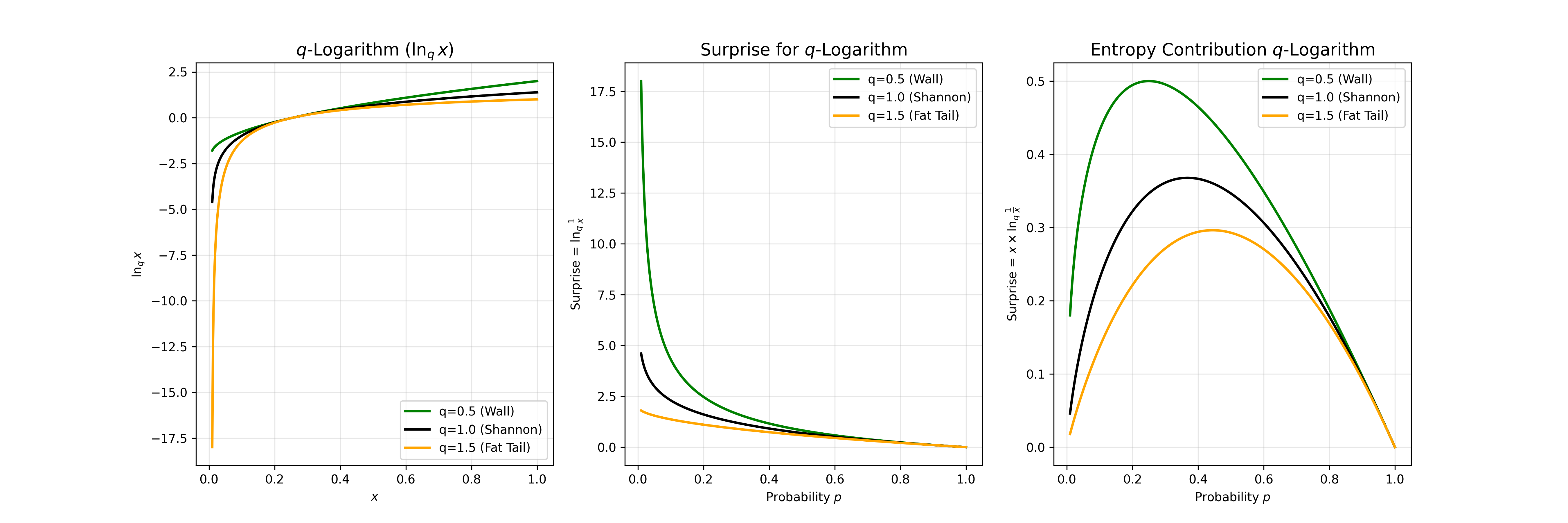
Let’s define the surprise (a.k.a information). To do that, we generalize the logarithm to a \(q\)-logarithm: \[ \ln_q x = \frac{x^{1-q} - 1}{1-q}. \]
It reduces to the usual log when \(q \to 1\). Its key algebraic property is a deformed additivity: \[ \ln_q(ab) = \ln_q a + \ln_q b + (1-q)\,\ln_q a \,\ln_q b. \]
Tsallis \( q \)-surprise is defined via the \(q\)-logarithm applied to the inverse probability: \[ I_q(x) = \ln_q \frac{1}{p(x)} = \frac{p(x)^{q-1} - 1}{1-q} = \frac{1 - p(x)^{q-1}}{q-1}. \]
Tsallis \( q \)-entropy is then just the average \(q\)-surprise: \[ S_q(A) = \sum_i p_i \ln_q \frac{1}{p_i} = \frac{1}{1-q}\left(\sum_i p_i^q - 1\right). \]
For \(q=1\), this smoothly recovers Shannon entropy.
In standard statistics, entropy adds up:\( S(A+B) = S(A) + S(B) \). However, in Tsallis-\( q \) statistics, entropy composition has a third interaction term: \(S(A+B) = S(A) + S(B) + \mathbf{(1-q) S(A) S(B)}\). The value of \( q \) acts as a knob that controls the strength of long-range interactions. Smaller \( q \) means the variables are more sparsely connected, while larger \( q \) increases their effective coupling.
-
The Standard World (\( q = 1 \)): The interaction term vanishes. Consider two decks of cards. If you shuffle one deck (\( S_A \)) and then shuffle a second deck (\( S_B \)), the total disorder is just the sum of both. They don’t magically interact.
-
The Structured World (\( q > 1 \)): \( (1-q) < 0. \) \( S(Total) < S(A) + S(B) \), i.e., the total mean surprise is less than the sum. Imagine the stock market activity of two groups: Technology traders and Silicon Chip traders. In normal times, they move somewhat independently. But when a rare event (a crash) hits, they suddenly lock together. The system shifts from many local events to one giant Super-Organism. This is the \( q>1 \) world. It allows for long-range correlations, meaning a small panic signal doesn’t die out; it travels across the “curved space” and aligns everyone instantly. In Shannon’s world, this synchronization is impossible because it assumes “distance creates independence”—the signal would have faded away before it could align the whole market.
-
The Explosive World (\( q < 1 \)): \( (1-q) > 0 \). \( S(Total) > S(A) + S(B) \). The total mean surprise is more than the sum. Imagine two people with different ideas. If they sit in separate rooms, they have 2 ideas. If they sit together, they talk, debate, and spark new ideas that neither had before. Language or social networks behave similarly. The connection creates “extra” possibilities that didn’t exist in the parts alone. This explosion of possibilities is also what creates sparsity in probability distribution.
Tsallis-q Constraints: Escort Averages and Variances
In the Tsallis world, there is a subtlety: if \(q > 1\), the distributions we expect are fat-tailed. In such worlds, the standard average \[ \langle E(x) \rangle = \sum_x p(x)\,E(x) \] can diverge (become infinite), because the tail is too heavy. This might remind you of the probability distributions where mean or variances are infinite.
To tame this, Tsallis-\( q \) statistics often uses escort averages: \[ \langle E(x) \rangle_q = \frac{\sum_x p(x)^q E(x)}{\sum_x p(x)^q}, \] and similarly an escort variance: \[ \mathrm{Var}_q(E) = \frac{\sum_x p(x)^q (E(x) - \mu)^2}{\sum_x p(x)^q}. \]
Because \(p(x)^q\) with \(q>1\) damps the tail more strongly (since \(p<1\)), these averages can remain finite even when the usual averages diverge. Interested readers can refer to the appendix to see why a standard (linear) average is not preferred in the Tsallis world.
\(q\)-Exponential Distribution
Maximize Tsallis-\( q \) entropy, \[ \max_{p} \frac{1 - \sum_i p_i^q}{q-1}, \] while enforcing two facts: \[ \sum_x p(x) = 1 \quad\text{(probabilities sum to one)},\qquad \sum_x p(x)E(x) = U \quad\text{(the average energy is fixed)}. \]
The Lagrangian is: \[ \mathcal{L} = \frac{1 - \sum_i p_i^q}{q-1} - \alpha\left(\sum_i p_i - 1\right) - \beta\left( \frac{\sum_i p_i^q E_i}{\sum_i p_i^q} - U_q \right). \]
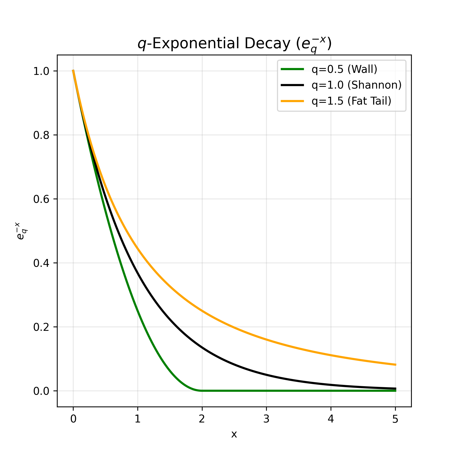
Solving this (Appendix B.2) gives the following form: \[ p(E) \propto \left[1 + (1-q)\,\tilde{\beta}\,(E - U_q)\right]^{\frac{1}{1-q}}, \] which is the \(q\)-exponential. For \(q>1\), this decays as a power law and yields genuine fat tails. For \(q<1\), the picture flips: the bracket can hit zero at a finite energy and then become negative, producing dead zones where the probability is effectively cut off yielding a sparse system.
Let’s introduce \( \text{exp}_q \) as the following function: \[ e_q^x = [1 + (1-q)x]^{\frac{1}{1-q}} \]
Then the \( q \)-exponential distribution can be written as: \[ p(x) \propto \text{exp}_q({-\frac{E(x)}{\beta}}) \]
\(q\)-Gaussian
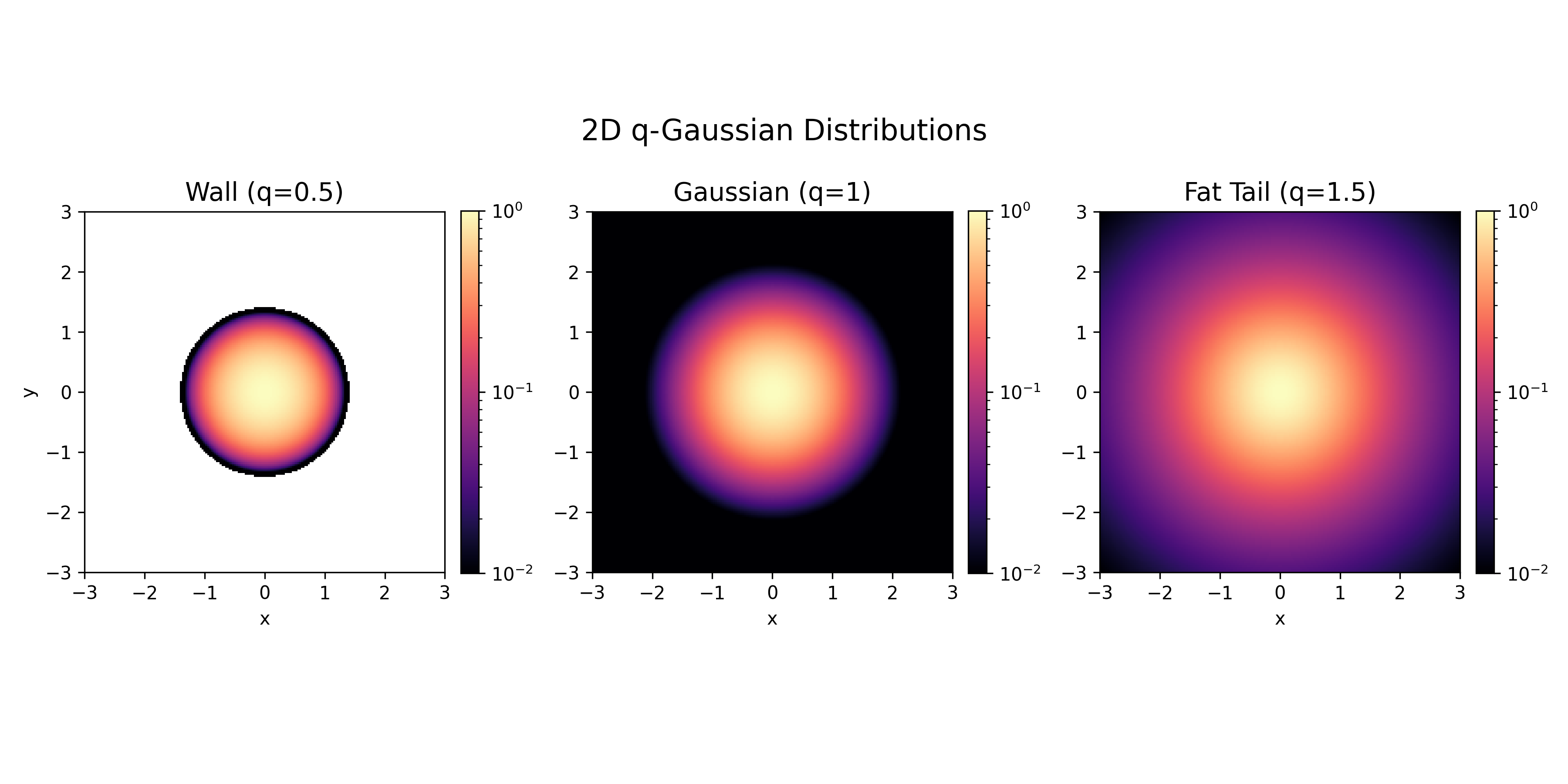
We can apply the same logic but with a escort variance constraint: \[ \frac{\sum_x p(x)^q (x-\mu)^2}{\sum_x p(x)^q} = \sigma_q^2. \]
The solution has the form: \[ p(x) \propto \left[1 + (1-q)\beta (x-\mu)^2\right]^{\frac{1}{1-q}}, \qquad \text{or} \qquad p(x) \propto \exp_q(\frac{(x-\mu)^2}{2\sigma_q^2}) \] often called a \(q\)-Gaussian. Note: as \(q \to 1\), this reduces to the standard Gaussian. The following plot reveals how \( q < 1 \) creates sparsity in the system or “Energy Wall”, whereas \( q > 1 \) creates systems with more variance than a normal Gaussian would.
Other Tsallis-\( q \) Max-Entropy distributions
| Name | Constraint / parameter regime | Form of \(p(x)\) (up to normalization) | Notes |
|---|---|---|---|
| \(q\)-Exponential | Escort mean energy fixed | \(p(x) \propto [1 + (q-1)\beta x]^{1/(1-q)}\) | Power-law relaxation instead of exponential. Seen in citation networks, re-tweets, and radioactive decay in porous media. |
| \(q\)-Gaussian | Escort variance fixed | \(p(x) \propto [1 + (q-1)\beta x^2]^{-1/(q-1)}\) | Generalized “bell curve”. Includes Gaussian as \(q\to 1\). |
| Cauchy (Lorentzian) | \(q=2\) case of \(q\)-Gaussian | \(p(x) \propto \dfrac{1}{1 + \gamma x^2}\) | Has infinite variance; very heavy tails. Represents a state where standard variance is infinite (undefined). It has the “fattest” possible tail before the normalization integral diverges. |
| Student’s t | \(q\)-Gaussian; \(1 < q < 3\), related to degrees of freedom \(\nu\) | \(p(x) \propto \left(1 + \nu x^2\right)^{-(\nu+1)/2}\) | Bridges Gaussian (\(\nu\to\infty\)) and Cauchy (\(\nu=1\)). \( \nu \) (degrees of freedom) measures uncertainty/correlation. \( \nu \rightarrow \inf: \) System is certain/independent. Limit is Gaussian (\( q \rightarrow 1 \)). \( \nu \rightarrow 1 \): System is uncertain/correlated. Limit is Cauchy (q→2). |
Why does CLT give a Gaussian?
One question that kept nagging me:
What is so special about variance constraints that when we add up many random variables, we get a Gaussian distribution (Central Limit Theorem)?
Mathematically, when you add two independent random variables \(Z = X + Y\), the distribution of \(Z\) is the convolution of the distributions of \(X\) and \(Y\).
Convolution acts like a blurring / smoothing operation.
- Start with a uniform distribution (a flat block). It has sharp corners.
- Add two uniforms: you get a triangle. Corners are softer.
- Add three: you get a smoother, almost parabolic shape.
- Keep adding: the shape smooths towards a Gaussian.
Visually, convolution keeps rounding off sharp features.
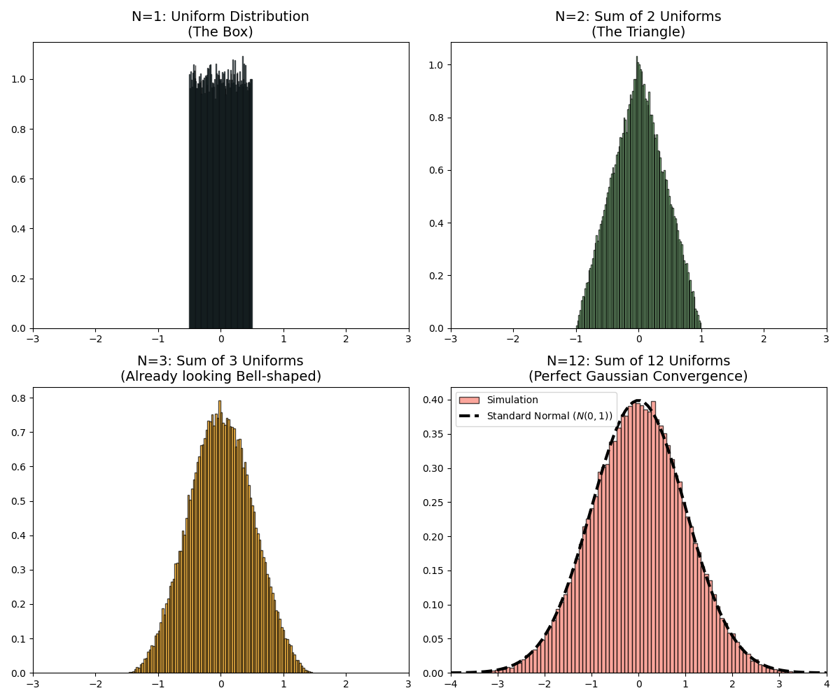
Why Gaussian in particular? Because the Gaussian is a fixed point of convolution under finite variance:
- The sum of two independent Gaussians is another Gaussian (just with a larger variance).
- So once the shape becomes “Gaussian enough”, further addition no longer change its shape.
Under mild conditions—independent variables, identical distribution, and finite variance—the classical Central Limit Theorem applies: repeated addition pushes almost any starting distribution toward a Gaussian. The Gaussian is the attractor in this finite-variance world.
In contrast, in the Tsallis / fat-tail world, where the variance is infinite, the assumptions of the usual CLT are violated. Here a generalized CLT holds instead, and the attractors become Lévy α-stable distributions, which have power-law tails.
Appendix
Tsallis-\( q \): Why standard mean constraint fails?
Maximize Tsallis entropy, \[ \max_{p} \frac{1 - \sum_i p_i^q}{q-1}, \] while enforcing two facts: \[ \sum_x p(x) = 1 \quad\text{(probabilities sum to one)},\qquad \sum_x p(x)E(x) = U \quad\text{(the average energy is fixed)}. \]
Lagrangian can be written as: \[ \mathcal{L} = \frac{1 - \sum_i p_i^q}{q-1} - \alpha\left(\sum_i p_i - 1\right) - \beta\left(\sum_i p_i E_i - U\right). \]
Derivative of the Lagrangian can be written as: \[ \frac{\partial \mathcal{L}}{\partial p_k} = -\frac{q\,p_k^{q-1}}{q-1} - \alpha - \beta E_k = 0. \]
Rearranging the terms: \[ \frac{q}{q-1} p_k^{q-1} = -\alpha - \beta E_k \quad\Rightarrow\quad p_k^{q-1} = A - B E_k, \] for some constants \(A,B\).
Thus: \[ p_k \propto \left(1 - \tilde{\beta} E_k\right)^{\frac{1}{q-1}}. \]
For \(q>1\), this is only defined for \(E_k < 1/\tilde{\beta}\), so the support is bounded, which is opposite of what we expect in \( q>1 \) because it exhibits long-range dependencies. With escort averages, we recover the expected behavior.
Deriving \(q\)-Exponential
Notice that we are still maximizing the average surprise and not the escort surprise. It is because probability is microscopic variable that we model, but the energy are macroscopic variables that we observe.
Maximize Tsallis entropy, \[ \max_{p} \frac{1 - \sum_i p_i^q}{q-1}, \] while enforcing two facts: \[ \sum_x p(x) = 1 \quad\text{(probabilities sum to one)},\qquad \frac{\sum p_i^q E_i}{\sum p_i^q} = U_q \quad\text{(the average energy is fixed)}. \]
The Lagrangian can be written as:\[\mathcal{L} = \frac{1 - \sum p_i^q}{q-1} - \alpha (\sum p_i - 1) - \beta \left( \frac{\sum p_i^q E_i}{\sum p_i^q} - U_q \right)\]
We take the derivative with respect to a specific probability \( p_k \) and set it to 0. Derivative of Entropy:\[\frac{\partial S_q}{\partial p_k} = \frac{-q p_k^{q-1}}{q-1}\] Derivative of Normalization:\[\frac{\partial}{\partial p_k} \alpha (\sum p_i - 1) = \alpha\] Derivative of Energy: \[\frac{\partial}{\partial p_k} \left( \frac{\sum p_i^q E_i}{\sum p_i^q} \right) = \frac{qp^{q-1}}{Z_q}(E_k - U_q)\]
Assembling the equation: \[\frac{qp^{q-1}}{Z_q}(E_k - U_q) + \beta \frac{qp^{q-1}}{1-q} - \alpha = 0\] Gathering terms so that only one element has constants: \[\frac{\beta qp^{q-1}}{1-q}[\frac{1-q}{\beta Z_q}(E_k - U_q) + 1] = \alpha\] Which yields a probability distribution like this: \[p \propto [1 + \beta^* (1-q)(E_k - U_q)]^{\frac{1}{1-q}}\]
Note for \( q > 1 \), this function is like \( y = \frac{1}{(1+x)^{\text{positive power}}} \). As \( E \to \infty \), the probability decays slowly but never hits zero.